Assessing Model Fit with Residual Plots
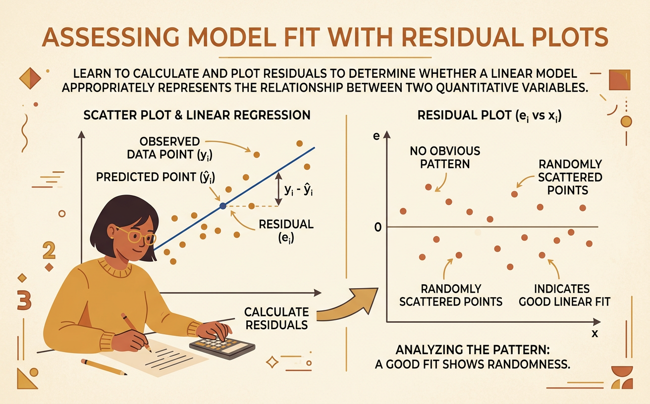
Students calculate and plot residuals to determine whether a linear model appropriately represents the relationship between two quantitative variables.
Illustrations are auto-generated and may be placeholders. They can be refreshed to match the narration.
Reviewing Predicted Values
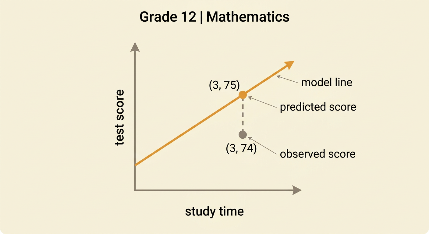
A predicted value is the response value produced by a model for a given explanatory value. Suppose a linear model relates weekly study time, x, to a test score, y. The model is predicted score = 5x + 60. To predict the score for a student who studies 3 hours, substitute 3 for x: predicted score = 5(3) + 60 = 75. Predicted values lie on the model’s line, while observed values are the actual scores recorded in the data. For study times of 1, 2, 3, 4, and 5 hours, the model predicts scores of 65, 70, 75, 80, and 85. Comparing these predictions with observed scores is the first step in assessing how well the linear model fits the data.
Calculating Residuals
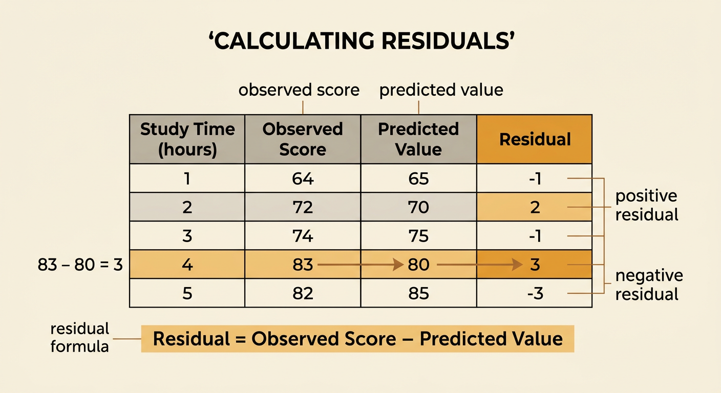
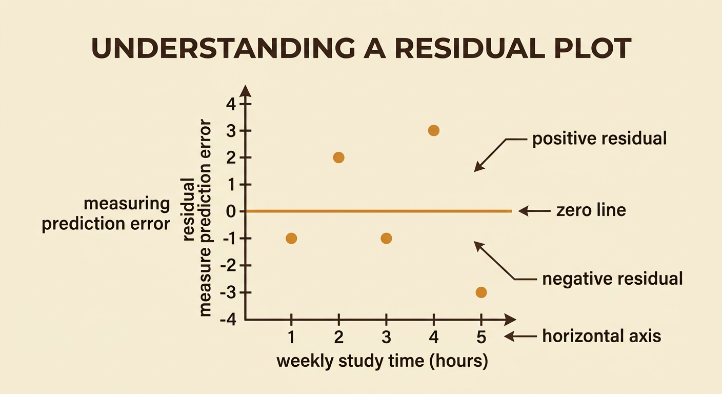
A residual measures the vertical difference between an observed value and the value predicted by a model. Calculate it using residual = observed value − predicted value. Consider observed test scores of 64, 72, 74, 83, and 82 for students who studied 1 through 5 hours. The model predicts 65, 70, 75, 80, and 85. Therefore, the residuals are −1, 2, −1, 3, and −3. A positive residual means the observed point is above the model’s line, so the model underestimated the response. A negative residual means the point is below the line, so the model overestimated the response. For example, at 4 hours, the observed score is 83 and the predicted score is 80. The residual is 83 − 80 = 3 points.
Creating a Residual Plot
A residual plot displays explanatory values on the horizontal axis and residuals on the vertical axis. Using the study-time data, plot the points (1, −1), (2, 2), (3, −1), (4, 3), and (5, −3). Draw a horizontal reference line at residual = 0. A point on this line represents a perfect prediction because the observed and predicted values are equal. Points above the line have positive residuals, and points below it have negative residuals. Keep the horizontal scale consistent with the original scatter plot, but replace test score on the vertical axis with residual. Do not connect the plotted points because each point represents a separate observation. The resulting graph makes the model’s prediction errors easier to inspect than a table of residual values alone.
Identifying Random and Systematic Patterns
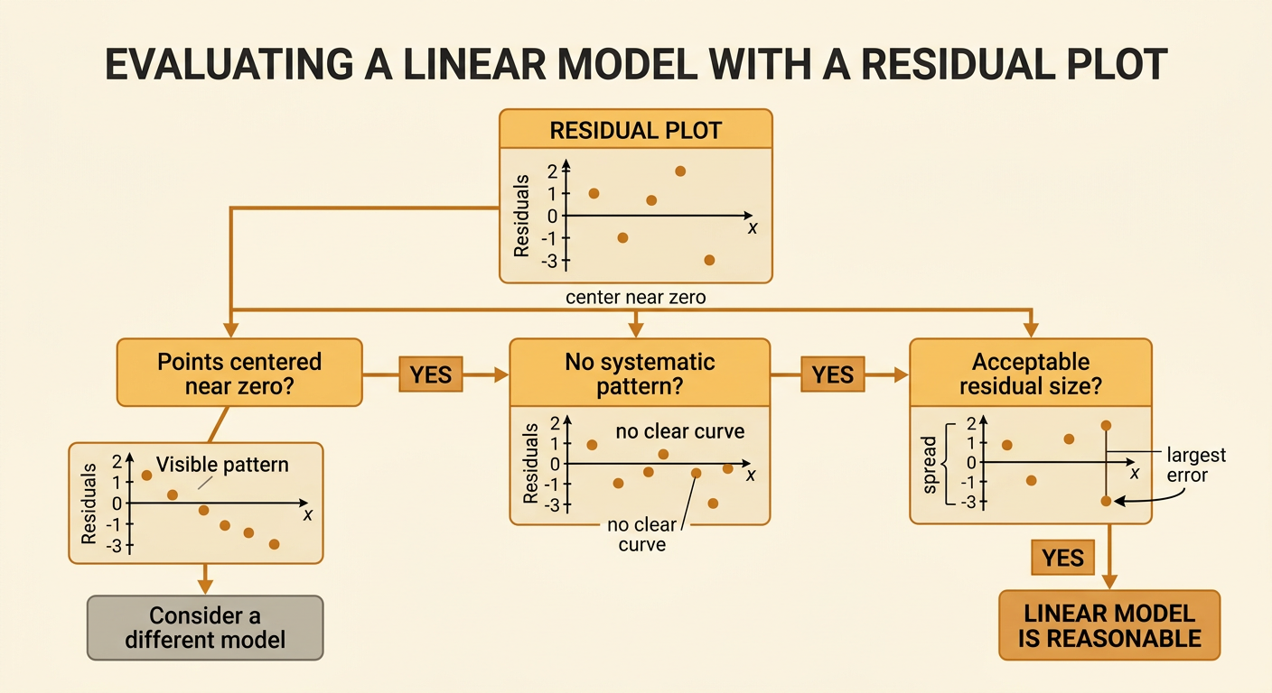
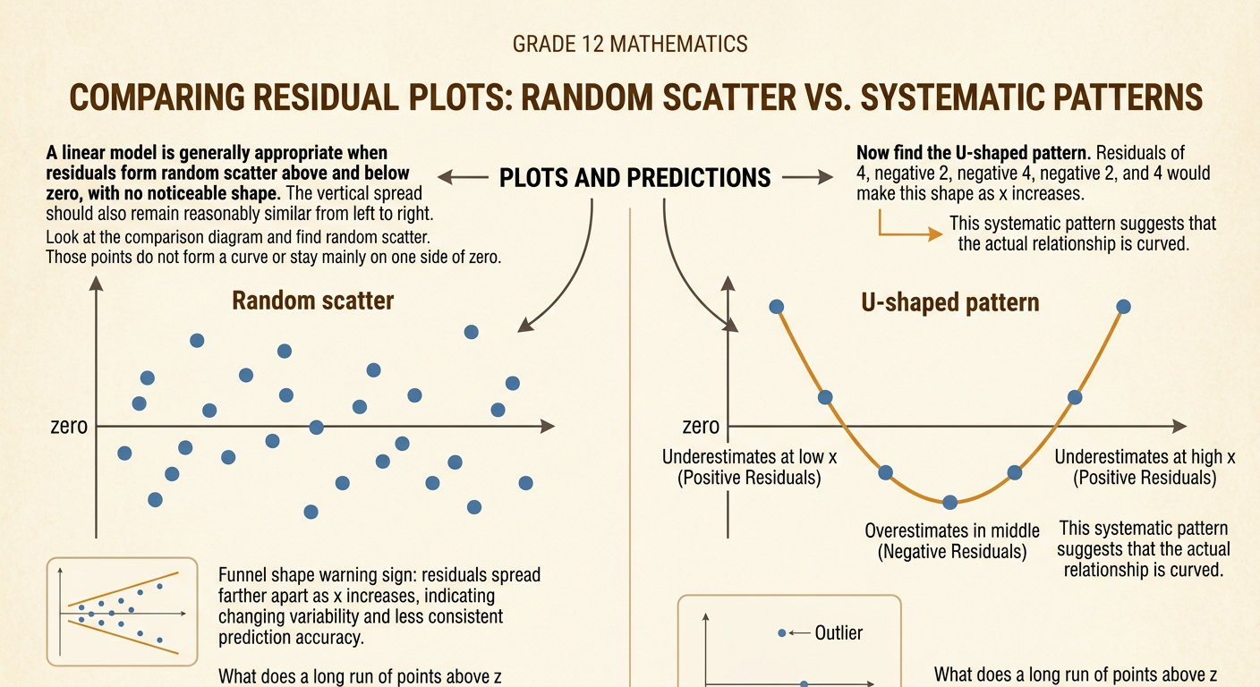
A linear model is generally appropriate when residuals are randomly scattered above and below zero without a noticeable shape. The vertical spread should also be reasonably similar across the horizontal axis. A systematic pattern suggests that the linear model misses an important feature of the relationship. For example, residuals of 4, −2, −4, −2, and 4 at increasing x-values form a U-shaped pattern. The model underestimates at low and high x-values but overestimates in the middle, indicating a curved relationship. A funnel shape, in which residuals spread farther apart as x increases, indicates changing variability. A long run of residuals on one side of zero also raises concern. Individual large residuals may identify outliers, but one unusual point alone does not necessarily make the entire linear model inappropriate.
Evaluating the Linear Model
To evaluate a linear model, consider the residual plot’s center, pattern, spread, and unusual points. Residuals should be centered near zero because a useful model should not consistently overpredict or underpredict. For the study-time example, the residuals −1, 2, −1, 3, and −3 occur on both sides of zero and show no clear curved pattern. Their magnitudes are at most 3 score points, which may be small enough for the intended use. Based on this limited sample, the linear model appears reasonable, although more observations would provide stronger evidence. If the residual plot showed a curve, a different function might fit better. If it showed increasing spread, predictions might become less reliable for larger x-values. A final conclusion should describe both the visible evidence and the practical size of the errors.