
Building and Validating a Computer Simulation
Students design a simple simulation with defined variables and rules, compare its output with reference data, and explain how assumptions affect the model’s reliability.

Illustrations are auto-generated and may be placeholders. They can be refreshed to match the narration.
Purpose of Computer Simulations
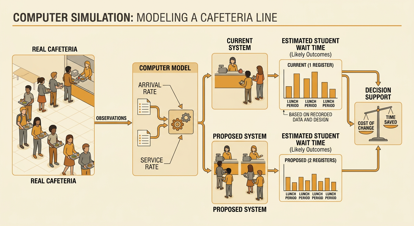
A computer simulation is an executable model of a real system. It uses selected features of that system to explore what may happen under different conditions. Simulations are useful when testing the real system would be expensive, slow, unsafe, or disruptive. For example, a school could simulate a cafeteria checkout line before paying to open a second register. The model might estimate student wait times using recorded arrival and service rates. Decision-makers could compare the current one-register system with a proposed two-register system across many simulated lunch periods. A simulation does not predict the future with certainty. Instead, it provides evidence about likely outcomes under stated conditions. Its usefulness depends on whether its variables, rules, assumptions, and input data represent the important parts of the real system.
Defining Variables, Rules, and Assumptions
Before coding, define the model's variables, rules, and assumptions. Input variables describe conditions supplied to the simulation, such as students arriving per minute, service time per student, lunch-period length, and number of registers. State variables change while the simulation runs, including current queue length and each register's availability. Output variables measure results, such as average wait time and maximum queue length. Rules specify behavior: arriving students join the shortest line, and an available cashier serves the first student waiting. Assumptions simplify reality. For example, the model may assume that no student leaves the line and that every register works continuously. These choices make the program manageable, but they can also make results less realistic. Each variable should have a unit, reasonable range, and source so that others can evaluate the model.

Coding the Simulation Loop
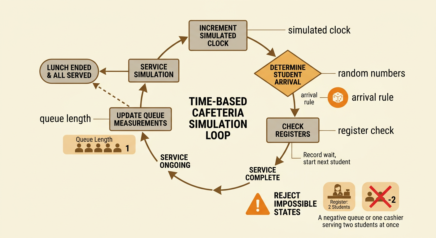
A simulation loop repeatedly updates the model as simulated time advances. In a cafeteria model, each loop iteration might represent one second. First, increase the simulated clock. Next, use the arrival-rate rule to determine whether a student enters the line. Then check each register. If a cashier has finished serving a student, record that student's wait and begin serving the next person in line. Finally, update queue length and other measurements. The loop continues until the lunch period ends and all remaining students are served. Random numbers can represent variation in arrivals and service times, but their probabilities should come from evidence rather than guesses. The program should also prevent impossible states, such as a negative queue length or one cashier serving two students at once. Small test cases help confirm that each rule works correctly.
Running and Recording Trials
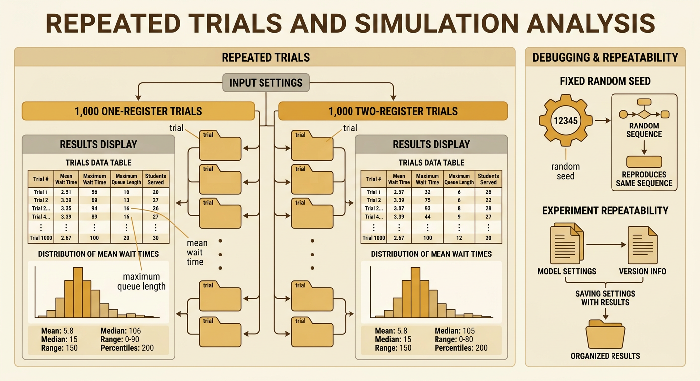
One simulation run is a trial, and a single trial may be unusual because random events vary. Therefore, run each proposed design many times under comparable conditions. For example, conduct 1,000 simulated lunch periods with one register and another 1,000 with two registers. Use the same arrival and service-time distributions for both scenarios so that the comparison is fair. For every trial, record outputs such as mean wait time, maximum wait time, maximum queue length, and the number of students served. Then summarize the trials with the mean, median, range, or selected percentiles. A fixed random seed can reproduce a run for debugging, while several different seeds provide broader evidence. Store the settings with the results so another person can repeat the experiment and determine exactly which version of the model produced each table or graph.
Validating Results with Reference Data
Validation asks whether simulation output agrees closely enough with trustworthy reference data for the model's intended use. Suppose observers timed waits during 20 real lunch periods with one register. Compare those observations with simulated one-register results using a table and graph. Check several measures, not just one average. If the observed mean wait is 6.2 minutes and the simulated mean is 6.0 minutes, the difference is 0.2 minute, but the model could still underestimate long waits. Compare medians, maximums, percentiles, and the shape of each distribution. An error measure such as mean absolute error can summarize typical differences between matched values. If adjustments are made using some observations, reserve different observations for final validation. This separation reduces the risk of tuning the model to one data set without improving its ability to represent other lunch periods.

Explaining Limitations and Reliability
Reliability describes how consistently and credibly a model supports conclusions for a stated purpose. It does not mean the model is perfectly accurate. The cafeteria simulation may omit students changing lines, cashier breaks, payment problems, or sudden arrivals after an assembly. Its reference data may also cover only a few days, making the estimated arrival rate uncertain. A strong evidence-based argument states the result, supporting data, assumptions, and weaknesses. For example, the trials may show that a second register usually reduces the median wait, supporting a limited trial of the change. A counterclaim might be that staffing costs outweigh the benefit or that unusual high-traffic days were not observed. Acknowledge that concern and identify needed evidence, such as more observations across different weeks. Conclusions should apply only to conditions the model represents, and sensitivity tests should show whether reasonable input changes alter the recommendation.
