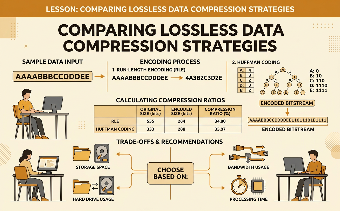
Comparing Lossless Data Compression Strategies
Students encode sample data, calculate compression ratios, and recommend a lossless compression strategy based on storage, bandwidth, and processing trade-offs.
Illustrations are auto-generated and may be placeholders. They can be refreshed to match the narration.
Why Compression Matters
Digital files consume storage space and network bandwidth. Lossless compression represents the same information with fewer bits while guaranteeing that the original data can be reconstructed exactly. This is essential for program files, financial records, scientific measurements, and text because even one changed value may cause an error. Suppose a school backs up 500 gigabytes of student projects. If lossless compression reduces the data to 300 gigabytes, the school stores and transfers 200 fewer gigabytes. That can lower storage fees and shorten upload time. However, compression and decompression also require processing time and energy. A useful strategy therefore depends on the data and the priorities. Repeated patterns may compress well, while random or previously compressed data may not. Engineers compare saved space and bandwidth with processing costs before selecting a method.

Lossless Encoding Rules
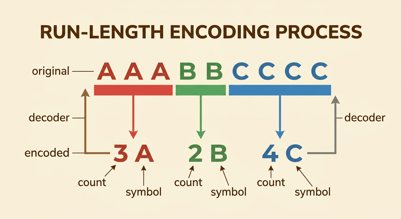
A lossless encoding rule must be reversible and unambiguous. The decoder must know where each encoded unit begins, what each value means, and when the data ends. In a simple run-length encoding format, each run is stored as a count followed by a symbol. For example, AAABBCCCC becomes 3A2B4C. The decoder reads 3A as three A symbols, 2B as two B symbols, and 4C as four C symbols, recreating AAABBCCCC exactly. A real file format might reserve one byte for each count and one byte for each symbol. It must also define how to handle runs longer than the largest count and symbols that are themselves digits. Headers, codebooks, and other decoding information must be included when measuring compressed size. Without those rules, a shorter representation may not be reliably reversible.
Trace Run-Length Encoding
Run-length encoding scans data from left to right and replaces each uninterrupted run with its length and symbol. Trace the string AAAABBCCCCCDAA. Begin with A and count until the symbol changes, producing 4A. The next run contains two B symbols, producing 2B. Five C symbols produce 5C. The single D produces 1D, and the final two A symbols produce 2A. The complete encoding is 4A2B5C1D2A. The original contains 14 symbols and the encoding contains five count-symbol pairs. If every original symbol uses one byte and every pair uses two bytes, the original requires 14 bytes while the encoding requires 10 bytes. Notice that the two A runs cannot be combined because they are separated by other symbols. Runs record consecutive repetition, not total frequency across the file.

Calculate Compression Ratios
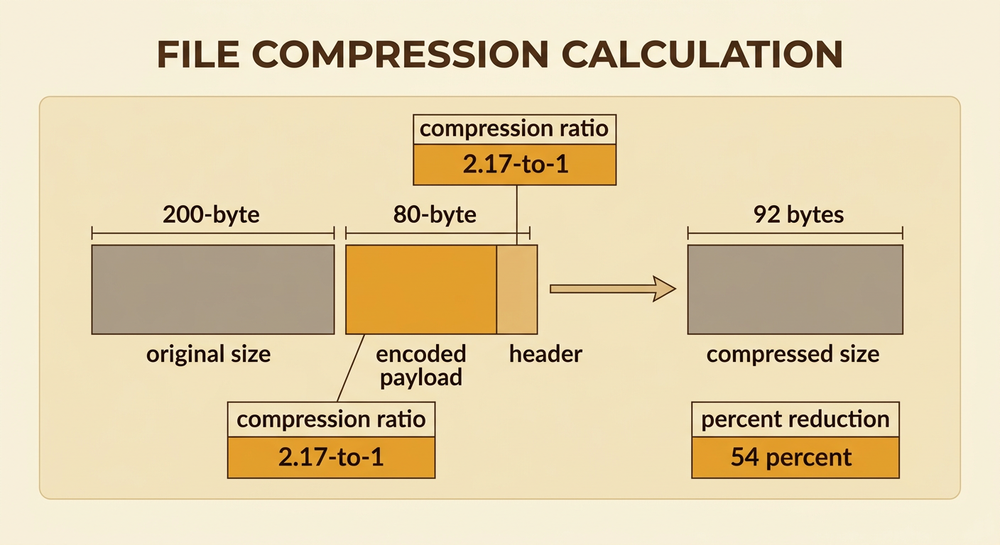
A compression ratio compares the original size with the complete compressed size. Using original size divided by compressed size, a 200-byte file compressed to 80 bytes has a ratio of 200 divided by 80, or 2.5 to 1. This means each compressed byte represents an average of 2.5 original bytes. Percent reduction is calculated as the original size minus the compressed size, divided by the original size, and multiplied by 100. The reduction is 120 divided by 200, or 60 percent. Always include required overhead. If the method also needs a 12-byte header, the total compressed size is 92 bytes. The adjusted ratio is about 2.17 to 1, and the reduction is 54 percent. Stating both the formula and included overhead makes comparisons fair and prevents an encoding from appearing more efficient than it really is.
Compare Costs and Benefits
The smallest output is not automatically the best choice because compression also uses processing time, memory, and energy. Consider a hypothetical organization that compresses 100 gigabytes of records to 60 gigabytes. If storage costs $0.02 per gigabyte each month, reducing 40 gigabytes saves $0.80 per month. If one network transfer costs $0.09 per gigabyte, the smaller file saves another $3.60 per transfer. The combined benefit for one month and one transfer is $4.40. If the extra computing required for compression and decompression costs $1.00, the net benefit is $3.40. More transfers increase the marginal benefit, while frequent recompression or expensive processing increases the marginal cost. Engineers should also compare nonfinancial constraints, such as maximum decoding time, available memory, battery use, and whether the data contains patterns that the method can exploit.

Recommend a Compression Method
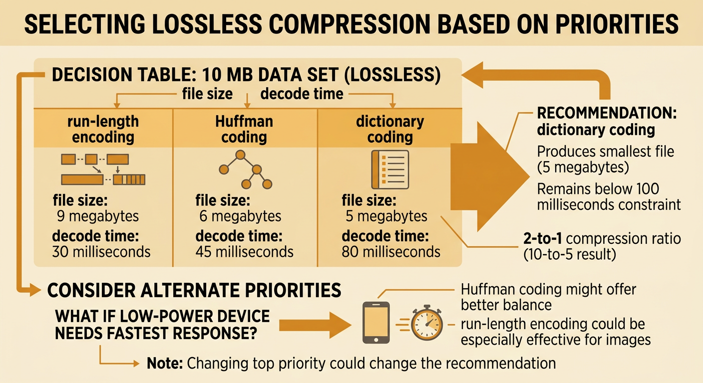
A recommendation should connect evidence to prioritized criteria and constraints. Suppose a 10-megabyte data set must remain lossless and decode in under 100 milliseconds. Tests show that run-length encoding produces 9 megabytes and decodes in 30 milliseconds, Huffman coding produces 6 megabytes and decodes in 45 milliseconds, and dictionary coding produces 5 megabytes and decodes in 80 milliseconds. All three satisfy the decoding constraint, but dictionary coding gives the greatest bandwidth and storage savings. If network transfer size is the highest priority, recommend dictionary coding and support the claim with its 2-to-1 compression ratio. If fast decoding on a low-power device becomes the highest priority, Huffman coding may offer a better balance, while run-length encoding may be preferred for images with very long repeated runs. A strong recommendation states the context, evidence, trade-offs, and conditions that could change the decision.