Comparing Sorting Algorithm Efficiency

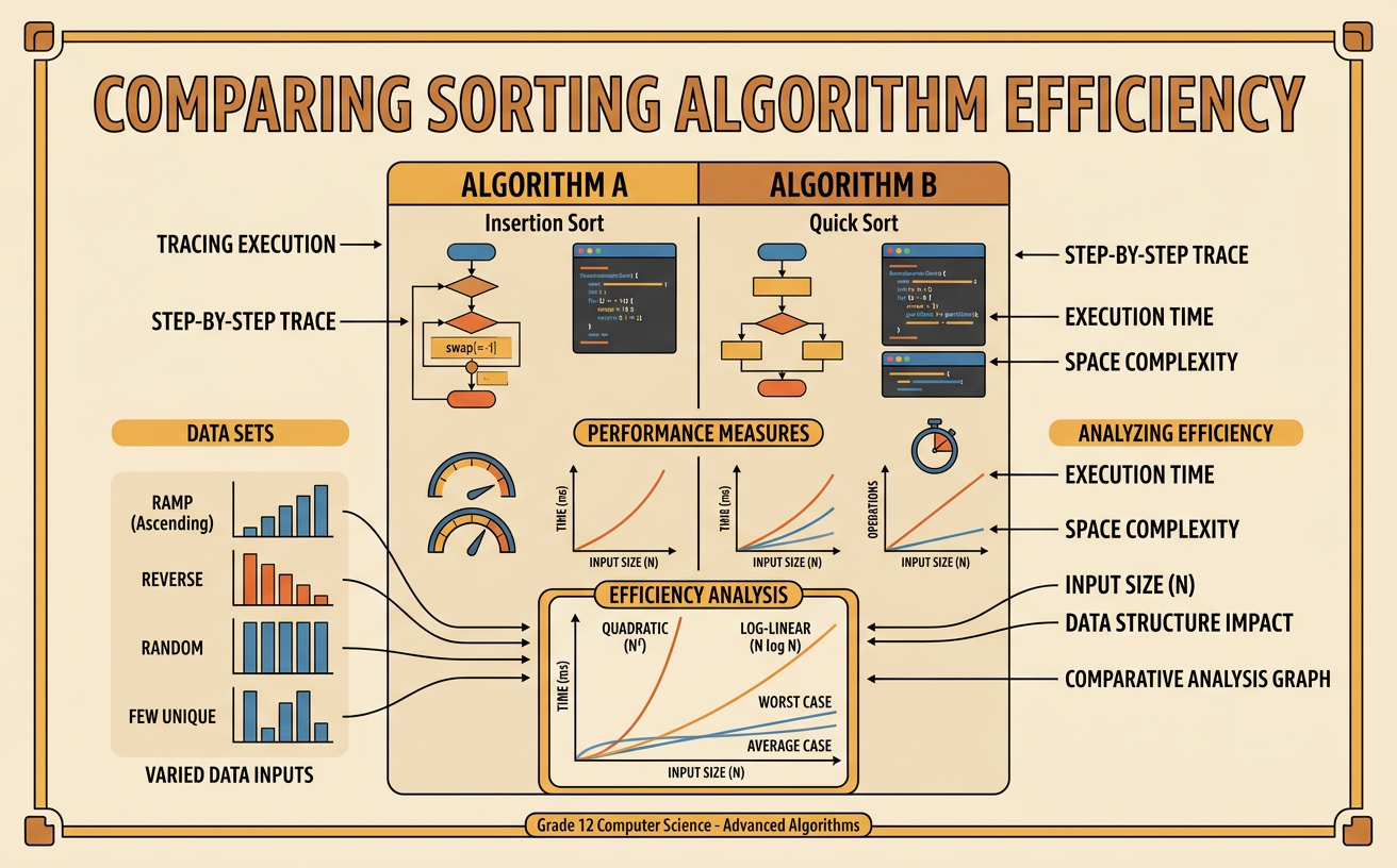
Students implement or trace two sorting algorithms, measure their performance on varied data sets, and use evidence to explain how input size and structure affect efficiency.

Sorting as a Computational Problem

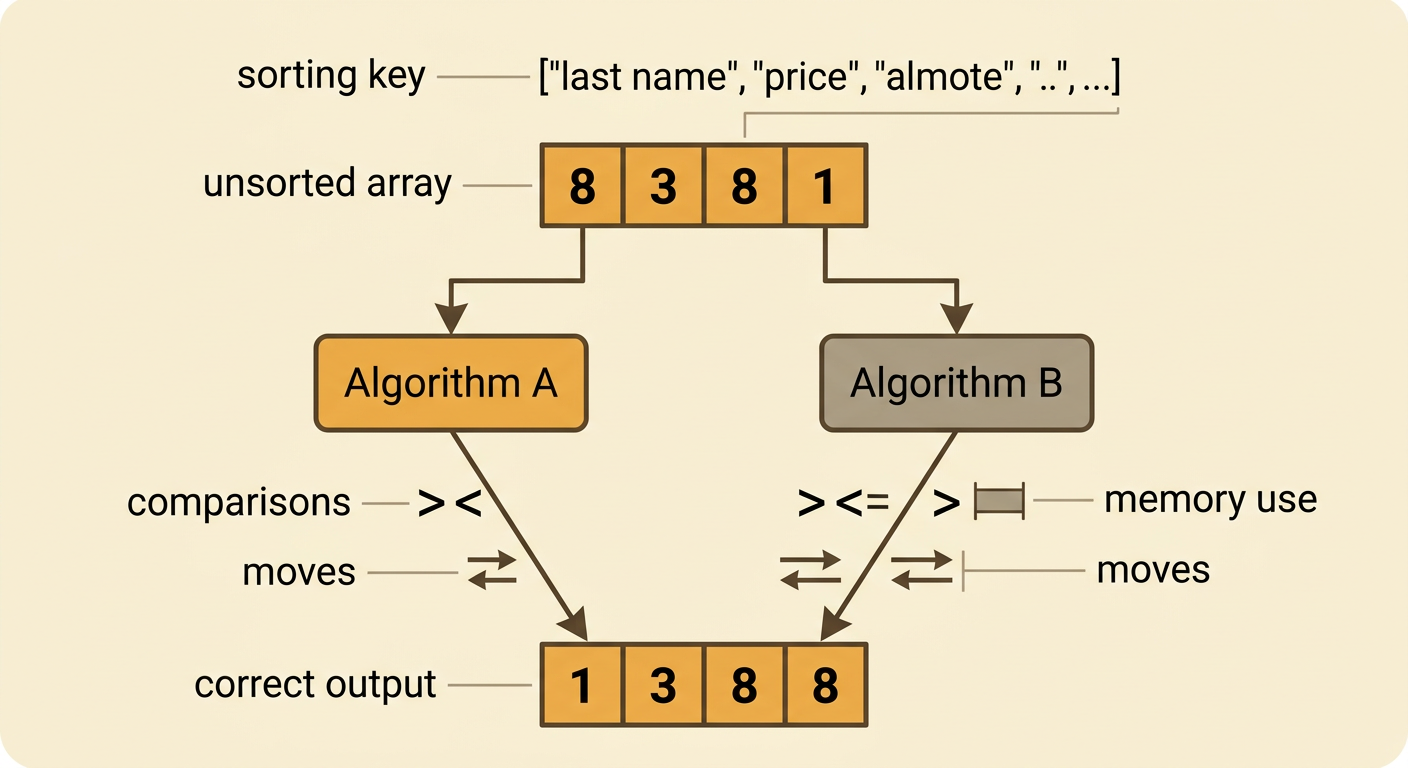
Sorting rearranges data according to a defined key, such as putting student records in order by last name or ranking products by price. A correct sorting algorithm must return every original item, place items in the requested order, and handle repeated values. Efficiency describes the resources used to produce that result. Important measures include elapsed time, number of comparisons, number of moves, and memory use. For example, sorting [8, 3, 8, 1] in ascending order should produce [1, 3, 8, 8]. Both copies of 8 must remain. Two algorithms can produce this same correct output while performing very different amounts of work. To compare them fairly, students should use identical inputs, the same computer and programming language, and clearly defined measurements. Correctness comes first; performance matters only after an algorithm reliably solves the problem.

Tracing Two Sorting Algorithms

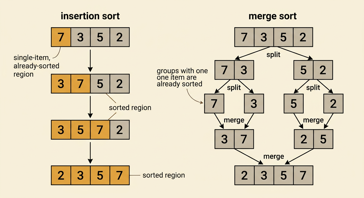
Insertion sort builds a sorted region one item at a time. For [7, 3, 5, 2], it inserts 3 before 7 to get [3, 7, 5, 2], inserts 5 between 3 and 7 to get [3, 5, 7, 2], and finally moves 2 to the front to get [2, 3, 5, 7]. Merge sort uses a different sequence. It divides the array into smaller halves until each part has one item, then merges the parts in order. It splits [7, 3, 5, 2] into [7, 3] and [5, 2], sorts them as [3, 7] and [2, 5], and merges them into [2, 3, 5, 7]. Tracing reveals where comparisons and moves occur. Recording each operation also helps verify correctness before timing the implementations.

Testing Different Inputs

A useful experiment changes both input size and input structure. Test each algorithm with random, already sorted, reverse-sorted, nearly sorted, and duplicate-heavy arrays. For example, create arrays of 100, 1,000, and 10,000 integers. A nearly sorted array might have only two values exchanged, while a duplicate-heavy array might contain values from 1 through 10 many times. Run both algorithms on exact copies so each receives the same data. Keep the computer, programming language, compiler settings, and measurement method constant. Repeat each trial several times and report the median elapsed time to reduce the effect of background processes. Also count comparisons or moves because clock measurements can vary. These controlled tests reveal whether an algorithm’s performance depends mainly on input size, on the arrangement of values, or on both factors.

Comparing Runtime and Scalability

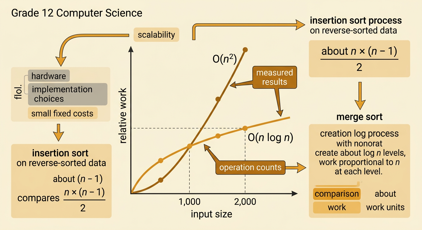
Scalability describes how resource use grows as the input becomes larger. Insertion sort has quadratic worst-case time, written O(n²), because a reverse-sorted input can require about n(n − 1) ÷ 2 comparisons. Merge sort runs in O(n log n) time across common input arrangements because it performs about log n levels of merging, with work proportional to n at each level. If input size doubles from 1,000 to 2,000, quadratic work grows by about four times. Work proportional to n log n grows by slightly more than two times. Actual milliseconds may not match these ratios exactly because hardware, implementation details, and small fixed costs matter. A graph of measured results should therefore be interpreted together with operation counts and growth-rate models. The trend across several input sizes is stronger evidence of scalability than one isolated timing result.

Evidence-Based Algorithm Selection

Choosing an algorithm requires prioritized criteria rather than declaring one method universally best. Relevant criteria may include runtime, memory use, stability, implementation complexity, and the expected input structure. Insertion sort is simple, uses little extra memory, and can perform well on small or nearly sorted data. Merge sort scales better for large, unpredictable inputs and is stable when implemented correctly, but array-based versions usually require additional temporary memory. Suppose a device repeatedly sorts 40 nearly ordered sensor readings under a strict memory limit. Test results may support insertion sort. A server sorting one million records may favor merge sort because scalability has higher priority. A strong recommendation combines code traces, measured trials, growth-rate analysis, and reliable technical documentation. It states the criteria, presents relevant evidence, explains trade-offs in logical order, and acknowledges limitations such as hardware differences or an unrepresentative test set.