
Conditional Probability and Independent Events
Students use two-way tables and probability rules to calculate conditional probabilities and determine whether two events are independent.
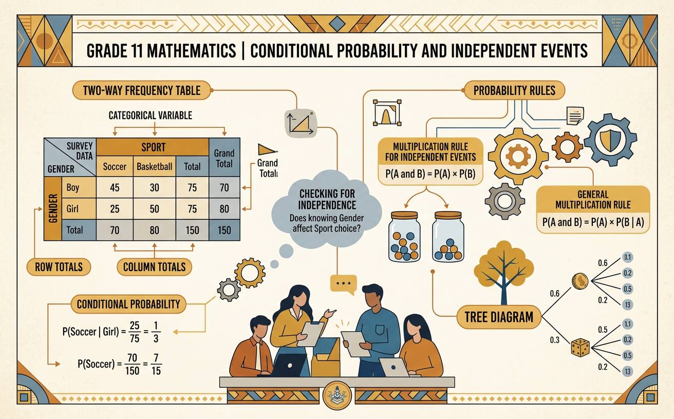
Illustrations are auto-generated and may be placeholders. They can be refreshed to match the narration.
Reviewing Compound Events
A compound event combines two or more events. The intersection of events A and B, written A and B, includes outcomes shared by both events. The union, written A or B, includes outcomes in either event or in both. For example, suppose one card is drawn from a standard 52-card deck. Let A be drawing a heart and B be drawing a face card. Three cards, the jack, queen, and king of hearts, belong to both events, so P(A and B) = 3/52. To find P(A or B), add the 13 hearts and 12 face cards, then subtract the 3 cards counted twice. Thus, P(A or B) = 22/52 = 11/26. The complement of A is not drawing a heart, with probability 39/52.

Reading Two-Way Tables
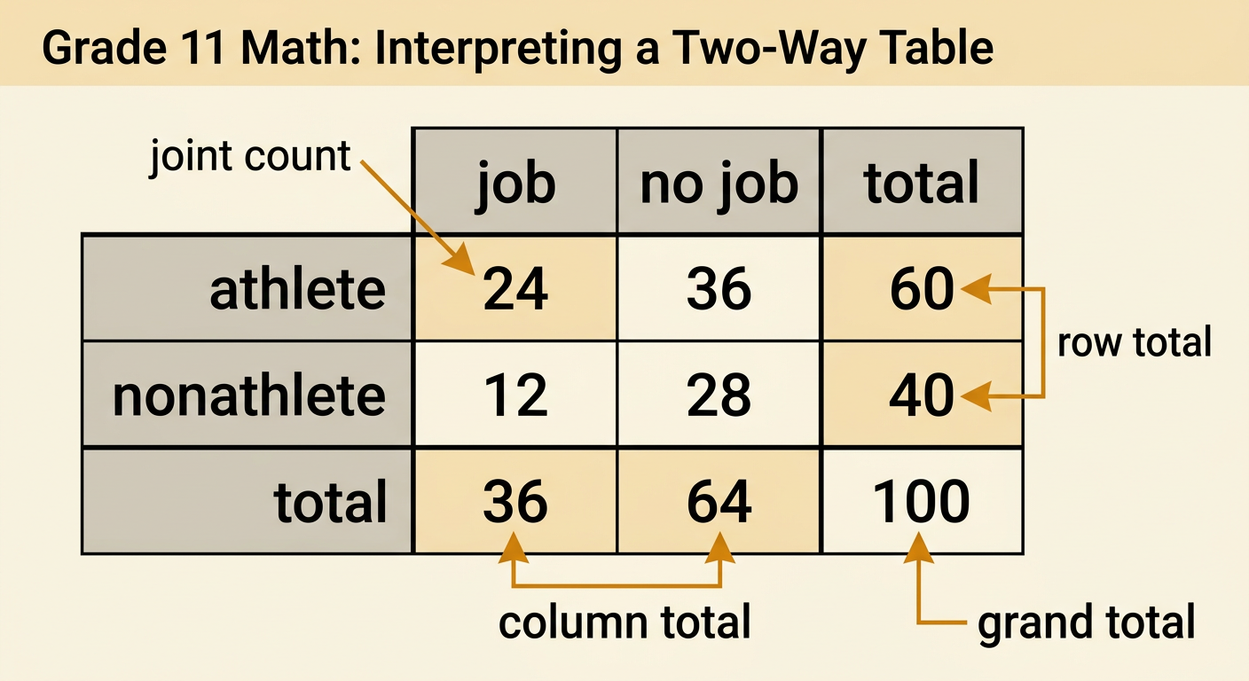
A two-way table organizes counts for two categorical variables and makes joint and marginal totals easy to compare. Suppose 100 students are classified by whether they play a school sport and whether they have a part-time job. Among 60 athletes, 24 have jobs and 36 do not. Among 40 nonathletes, 12 have jobs and 28 do not. The joint count for being an athlete and having a job is 24. Row totals show that 60 students are athletes and 40 are not. Column totals show that 36 students have jobs and 64 do not. The grand total is 100. A probability based on the entire group uses the grand total as its denominator. For example, P(athlete and job) = 24/100 = 0.24, while P(job) = 36/100 = 0.36.
Calculating Conditional Probability
Conditional probability measures the chance that one event occurs when another event is already known to have occurred. The notation P(A given B) means the probability of A under the condition B. Use the rule P(A given B) = P(A and B) divided by P(B), provided P(B) is not zero. In the student table, suppose a student is known to be an athlete. This condition limits the sample space from all 100 students to the 60 athletes. Of those 60 athletes, 24 have part-time jobs. Therefore, P(job given athlete) = 24/60 = 0.40. Reversing the condition gives a different calculation: among the 36 students with jobs, 24 are athletes, so P(athlete given job) = 24/36, or about 0.67. The order of the events matters because the condition determines the denominator.

Testing Events for Independence
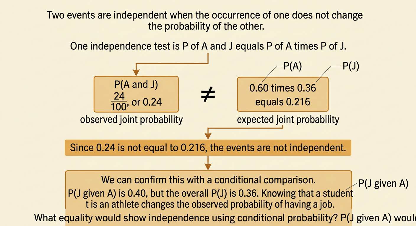
Two events are independent when the occurrence of one event does not change the probability of the other. Events A and B are independent if P(A and B) = P(A) times P(B). They are also independent if P(A given B) = P(A), when P(B) is greater than zero. Using the student data, let A be being an athlete and J be having a job. The table gives P(A) = 60/100 = 0.60 and P(J) = 36/100 = 0.36. If the events were independent, their joint probability would be 0.60 times 0.36, or 0.216. However, the observed joint probability is P(A and J) = 24/100 = 0.24. Because 0.24 is not equal to 0.216, the events are not independent. Equivalently, P(J given A) = 0.40 differs from P(J) = 0.36.
Applying Probability to Real-World Data
Conditional probability can reveal an association in real-world data. Suppose a school surveys 200 students about attending a review session and passing a mathematics exam. Of 80 students who attended, 68 passed and 12 did not. Of 120 students who did not attend, 78 passed and 42 did not. The overall pass rate is 146/200 = 0.73. The conditional pass rate for attendees is 68/80 = 0.85, while the rate for nonattendees is 78/120 = 0.65. Because attending changes the observed conditional probability of passing, attendance and passing are not independent in this data set. The product test confirms this: P(attend) times P(pass) = 0.40 times 0.73 = 0.292, but P(attend and pass) = 68/200 = 0.34. This association does not by itself prove that attending caused higher scores.