
Developing and Using Probability Models
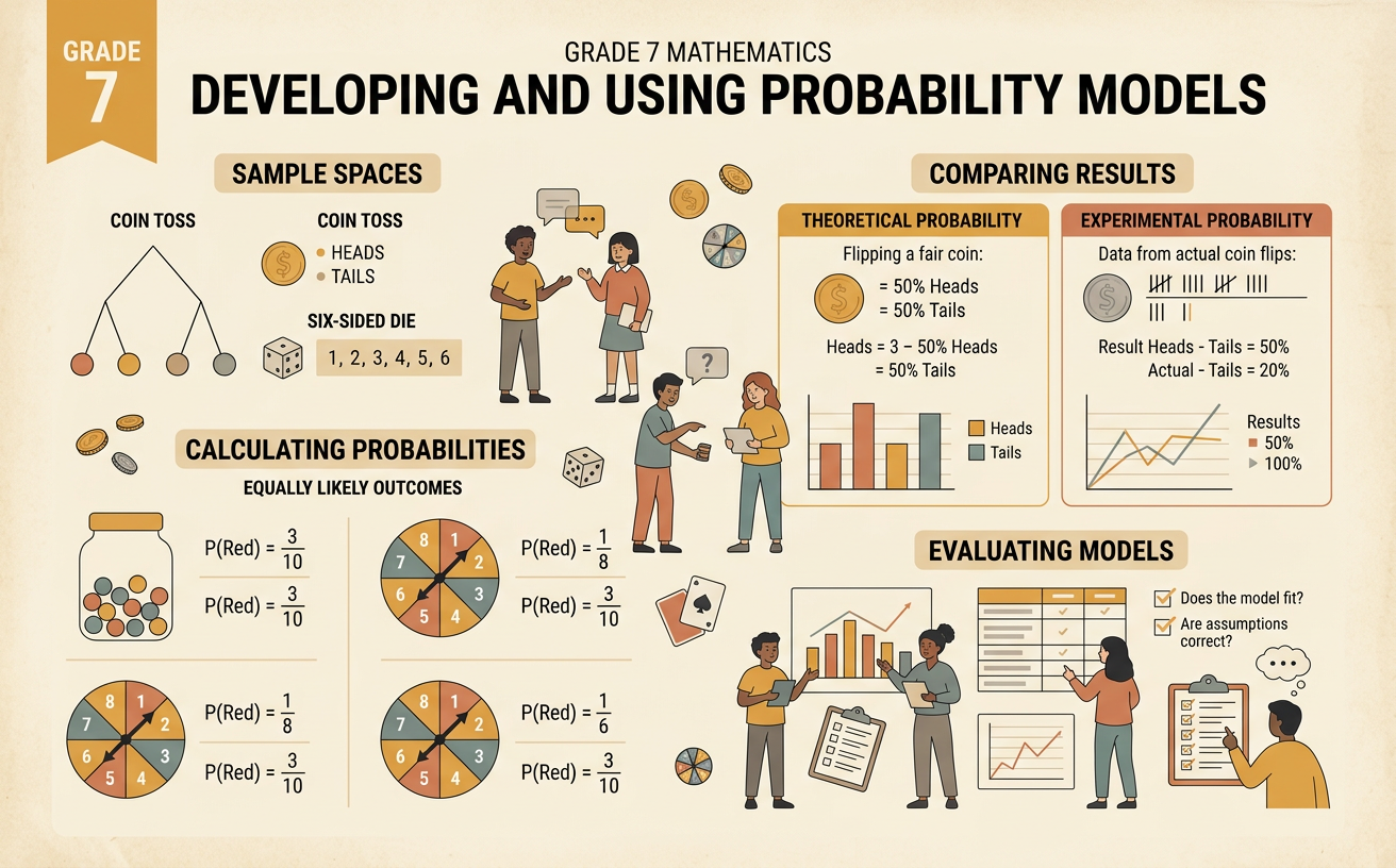
Students describe sample spaces, calculate probabilities for equally likely outcomes, compare theoretical and experimental results, and evaluate probability models.
Illustrations are auto-generated and may be placeholders. They can be refreshed to match the narration.
Chance Events and Sample Spaces
A chance event has an outcome that is uncertain before an experiment occurs. The sample space is the set of all possible outcomes. When a standard number cube is rolled, the sample space is 1, 2, 3, 4, 5, and 6. An event is one or more outcomes from that sample space. The event of rolling an even number contains 2, 4, and 6. Listing the complete sample space prevents possible outcomes from being overlooked. For a spinner with red, blue, green, and yellow sections, the sample space contains those four colors. If the spinner sections are equal in size, the outcomes are equally likely. If the sections differ in size, simply counting the colors is not enough; the size of each section must be considered when developing the probability model.
Probability as a Number from Zero to One
Probability measures how likely an event is and ranges from 0 to 1. A probability of 0 describes an impossible event, while a probability of 1 describes a certain event. Values closer to 1 indicate greater likelihood. For equally likely outcomes, probability equals the number of favorable outcomes divided by the total number of possible outcomes. On a fair six-sided number cube, the probability of rolling a number greater than 4 is 2 out of 6 because 5 and 6 are favorable. This simplifies to one third. The probability may also be written as a decimal or percent, such as approximately 0.333 or 33.3 percent. The probability of not rolling a number greater than 4 is four sixths, or two thirds. An event and its complement always have probabilities that add to 1.
Building Models for Equally Likely Outcomes
A probability model lists each outcome and assigns a probability to it. For a fair coin, heads and tails each have probability one half. For a bag containing three identical red counters and two identical blue counters, each individual counter is equally likely to be selected. The probability of red is three fifths, and the probability of blue is two fifths. These probabilities add to 1 because the model includes every possible color outcome. Tables, organized lists, and diagrams can display probability models clearly. Suppose a fair spinner has eight equal sections: three orange, four purple, and one white. The model assigns probability three eighths to orange, four eighths to purple, and one eighth to white. The physical structure of the experiment justifies the probabilities rather than a guess about which outcome seems likely.
Experimental and Theoretical Probability
Theoretical probability is based on a model of how an experiment should behave. Experimental probability is based on observed results. If a fair coin is flipped 50 times and lands on heads 28 times, the experimental probability of heads is 28 divided by 50, or 0.56. The theoretical probability remains 0.5. A difference between the two does not necessarily mean the coin is unfair. Random variation is common in a small number of trials. As the experiment is repeated many more times, the experimental relative frequency often moves closer to the theoretical probability. For example, after 1,000 flips, a result near 500 heads would be expected. Comparing theoretical and experimental values helps determine whether a model is reasonable or whether factors such as an uneven spinner or biased selection may affect results.
Models with Unequally Likely Outcomes
Not all outcomes are equally likely. Imagine a spinner divided into four regions: one half is blue, one fourth is red, and the remaining two eighth-sized regions are green and yellow. Although there are four color outcomes, each does not have probability one fourth. Blue has probability one half, red has probability one fourth, and green and yellow each have probability one eighth. The probabilities still add to 1. Data can also be used to create a model when the physical probabilities are unknown. If a machine produces 70 acceptable items and 30 defective items in a sample of 100, a data-based model estimates probabilities of 0.70 and 0.30. The model should be revised if more trials produce substantially different relative frequencies. A useful model matches the experiment's structure or reliable long-term data.