
Estimating Population Parameters with Margin of Error
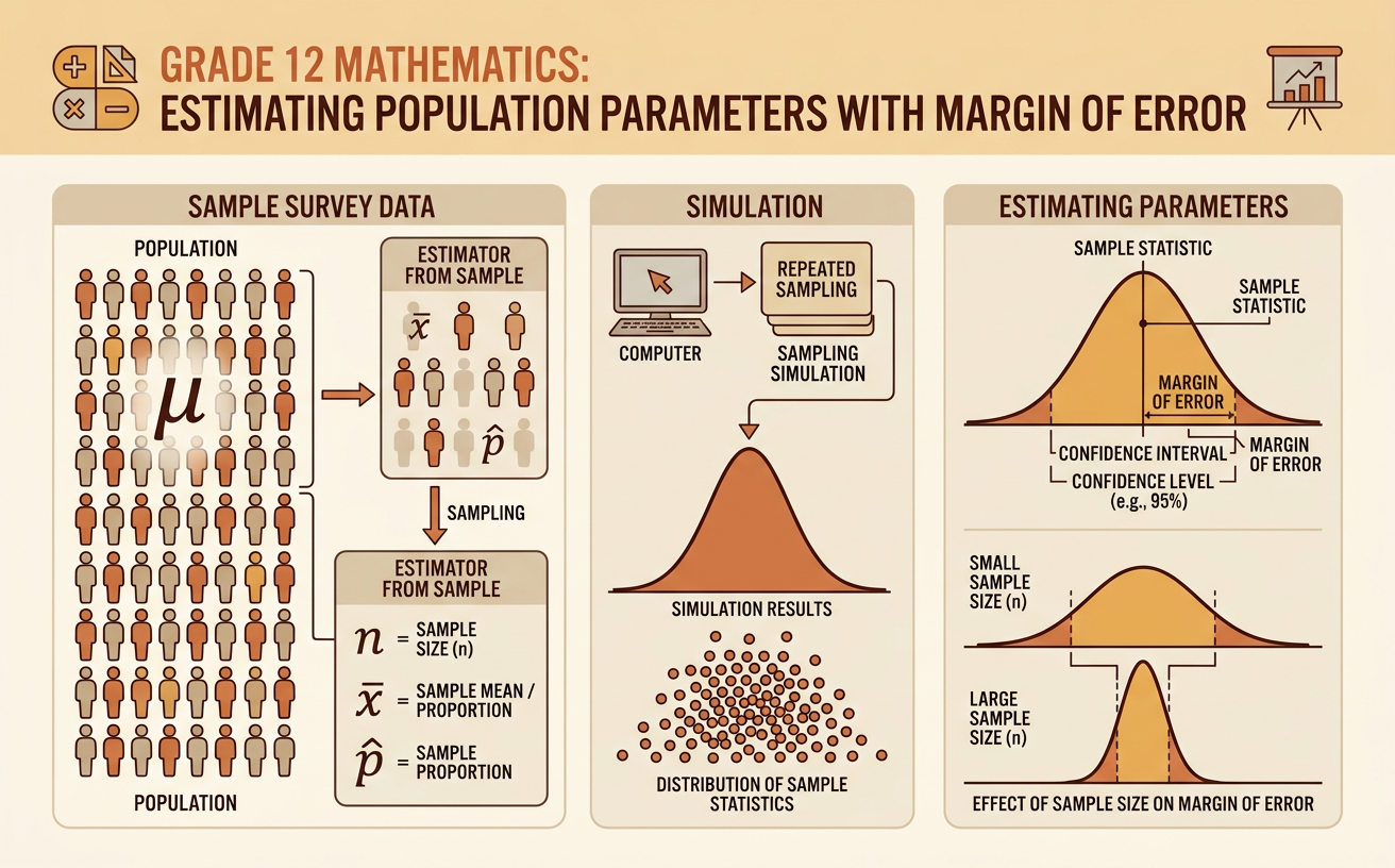
Students use sample survey data and simulation to estimate a population mean or proportion and explain how sample size affects margin of error.
Illustrations are auto-generated and may be placeholders. They can be refreshed to match the narration.
From Samples to Populations
A population is the entire group a study seeks to describe, while a sample is the smaller group from which data are collected. Because surveying every member of a population may be costly or impossible, researchers use a sample to make an inference about the population. Suppose a school district wants to know what proportion of its 4,000 seniors support a later start time. Researchers randomly select 200 seniors and record their responses. If the selection process gives every senior a fair chance of being chosen, the sample can provide useful evidence about all district seniors. A large sample does not automatically guarantee accuracy. A voluntary online poll, for example, may overrepresent students with strong opinions. Random selection reduces selection bias and makes margin-of-error calculations meaningful.

Point Estimates
A point estimate is a single value calculated from a sample and used to estimate an unknown population parameter. For categorical data, the sample proportion, written as p-hat, estimates the population proportion. If 118 of 200 surveyed seniors support a later start time, then p-hat equals 118 divided by 200, or 0.59. The point estimate is therefore 59%. For numerical data, the sample mean, written as x-bar, estimates the population mean. If a random sample of seniors reports an average of 6.8 hours of sleep per night, then 6.8 hours is the point estimate of the population mean. Point estimates are unlikely to equal the parameter exactly because different random samples produce different results. Margin of error describes the likely size of this sampling variation.

Simulating Random Samples
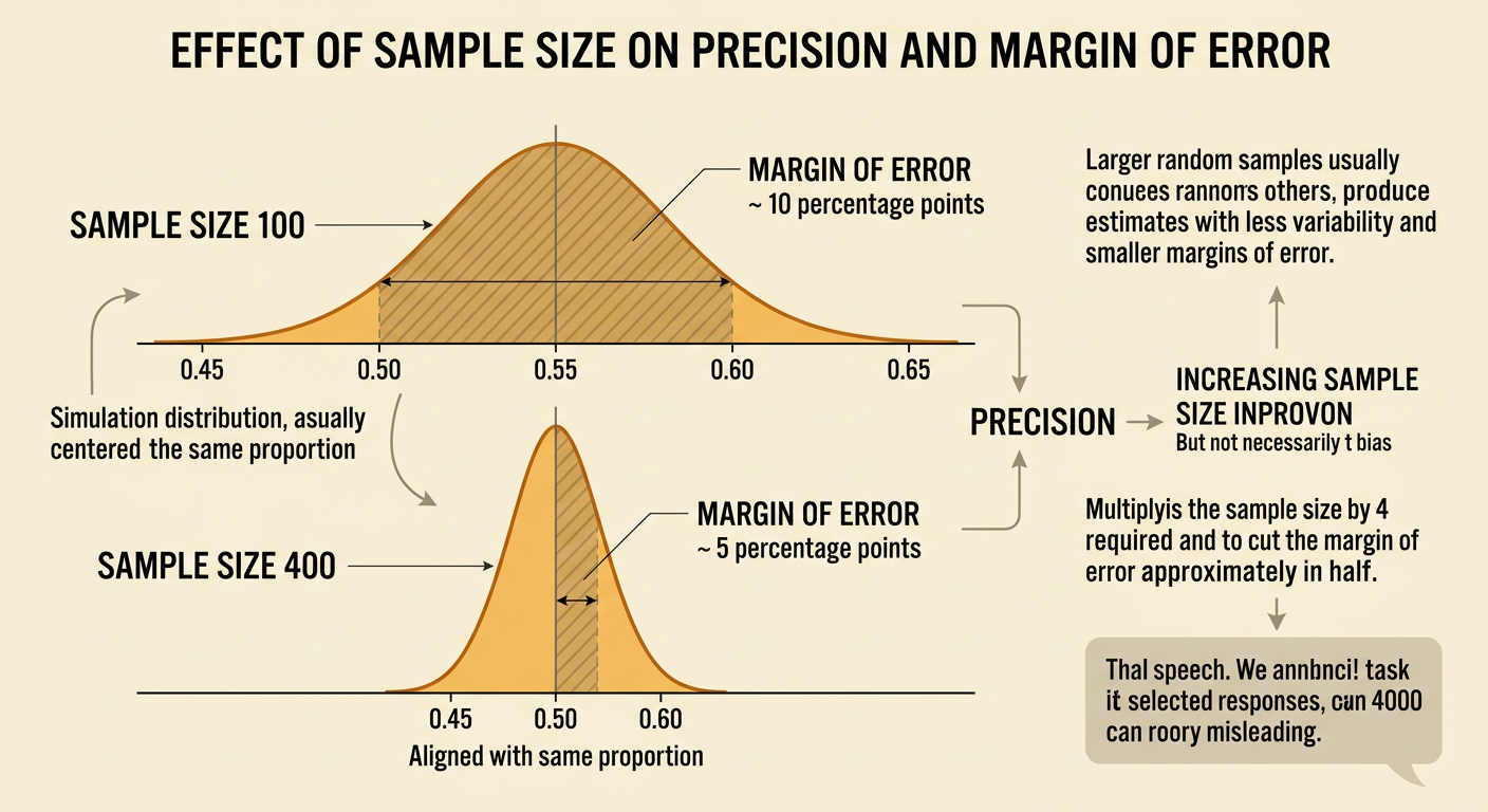
Simulation reveals how much an estimate can vary from sample to sample. Begin with a model population, or use the observed sample as an approximation of the population. Then repeatedly draw random samples of the same size and calculate the statistic for each sample. Suppose 55% of a sample of 100 students favor a proposal. A computer can model a population with a 0.55 support rate, draw thousands of random samples of 100, and record every sample proportion. The resulting distribution will be centered near 0.55, but individual results will vary. About 95% may fall roughly between 0.45 and 0.65. The distance from the center to either endpoint, about 0.10, provides a simulation-based margin of error of approximately 10 percentage points.

Interpreting Margin of Error
Margin of error gives a range of plausible values around a point estimate under a specified simulation method and confidence level. If 55% of surveyed students support a proposal and the simulated margin of error is 10 percentage points, the interval is 55% plus or minus 10 percentage points, or 45% to 65%. This does not mean that exactly 95% of students fall in the interval. It means that a method producing 95% intervals would capture the true population proportion in about 95% of many repeated random samples. The population parameter is fixed; the interval changes from sample to sample. Margin of error accounts for random sampling variation, but it does not correct biased questions, nonresponse, inaccurate answers, or a sample that was not randomly selected.

Effect of Sample Size
Larger random samples usually produce less variable estimates and smaller margins of error. For many common sampling situations, margin of error changes approximately in proportion to one divided by the square root of the sample size. Therefore, doubling the sample size does not cut the margin of error in half; the sample size must be multiplied by four to do that. For example, simulations for samples of 100 students might produce a margin of error near 10 percentage points. Under similar conditions, samples of 400 students might produce a margin of error near 5 percentage points. A simulation plot for 400 observations will be narrower than one for 100 observations. Increasing sample size improves precision, but it cannot repair a biased sampling method. A carefully selected random sample is still essential.
Communicating Conclusions
A strong statistical conclusion identifies the population, sampling method, point estimate, margin of error, and practical limitations. Suppose a random sample of 200 district seniors reports a mean of 6.8 hours of sleep per night. A simulation produces a margin of error of 0.4 hour at the 95% level. An appropriate conclusion is: We estimate that district seniors average between 6.4 and 7.2 hours of sleep per night, based on a random sample and a simulation-based 95% margin of error. The conclusion should not claim that every senior sleeps within this range; the interval estimates the population mean, not individual values. It should also mention possible nonresponse or inaccurate self-reports. Conclusions apply only to the population from which the random sample was selected and do not establish cause and effect.