Evaluating a Machine Learning Classifier

Students interpret a confusion matrix, calculate classification metrics, and examine how training data quality can affect a model’s accuracy and fairness.

How Classifiers Make Predictions

A machine learning classifier assigns an input to a category. During training, it examines labeled examples and identifies patterns in features, which are measurable characteristics of the examples. For instance, an email spam classifier might use the sender, number of links, and presence of certain words as features. For a new email, the model produces a score representing how strongly the email matches learned spam patterns. A decision threshold converts that score into a prediction: spam or not spam. The prediction is not proof that the model understands the message. It is a result based on patterns in its training data. To evaluate the classifier, developers compare its predictions with verified labels in a separate test data set that was not used for training.

Reading a Confusion Matrix

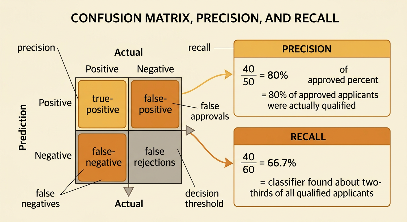
A confusion matrix is a two-way frequency table that compares predicted categories with actual categories. Consider a loan classifier tested on 100 applicants whose qualifications were independently verified. It approved 40 qualified applicants, called true positives, and rejected 30 unqualified applicants, called true negatives. It also approved 10 unqualified applicants, producing false positives, and rejected 20 qualified applicants, producing false negatives. The rows can represent actual status, while the columns represent the model’s prediction. Correct results appear in the true-positive and true-negative cells. Errors appear in the other two cells. The matrix reveals information that one overall score can hide. In this example, the model made 70 correct predictions out of 100, so its accuracy was 70 percent, but it still denied 20 qualified applicants.

Calculating Precision and Recall

Precision and recall answer different questions about a classifier’s positive predictions. Precision is true positives divided by all predicted positives. In the loan example, the model approved 50 applicants: 40 qualified and 10 unqualified. Its precision was 40 divided by 50, or 80 percent. This means 80 percent of approved applicants were actually qualified. Recall is true positives divided by all actual positives. There were 60 qualified applicants, and the model approved 40 of them. Its recall was 40 divided by 60, or about 66.7 percent. This means the model identified about two-thirds of all qualified applicants. Raising a decision threshold often increases precision but decreases recall because the model makes fewer positive predictions. The preferred balance depends on the consequences of false approvals and false rejections.

Investigating Training Data Quality

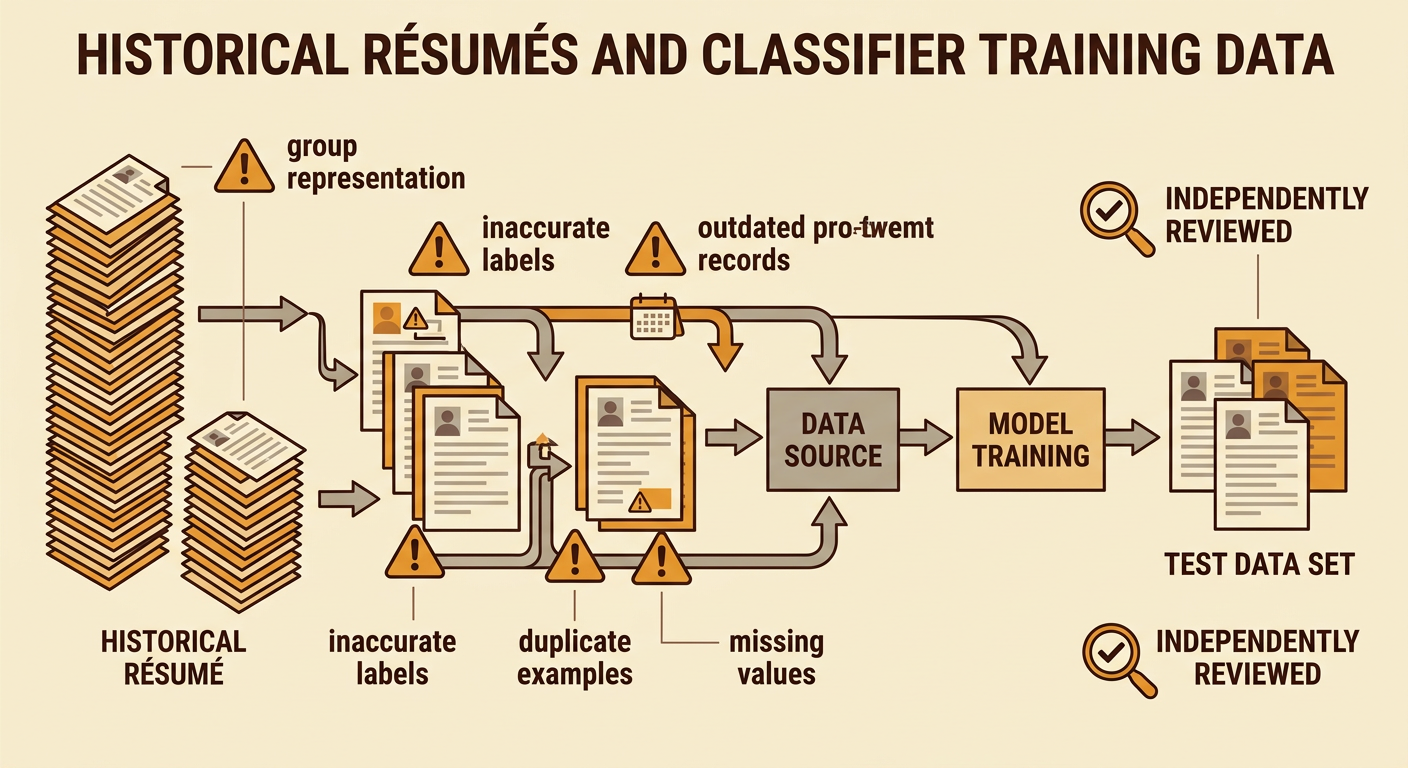
A classifier can reproduce weaknesses in its training data. Investigators should examine the data’s origin, who collected and labeled it, why it was created, which groups are represented, and whether other credible sources corroborate it. Suppose a hiring classifier is trained mainly on résumés from past employees at a company that historically hired few women for technical roles. The model may learn that patterns associated with men are linked to hiring, even when gender is not an explicit feature. Inaccurate labels, outdated records, duplicate examples, missing groups, and measurements that serve as poor substitutes for job ability can also reduce quality. Developers should document the source, test label consistency, look for missing values, compare group representation, and evaluate results on recent, independently reviewed data. More data does not solve a problem if the additional data repeats the same bias.

Comparing Accuracy and Fairness

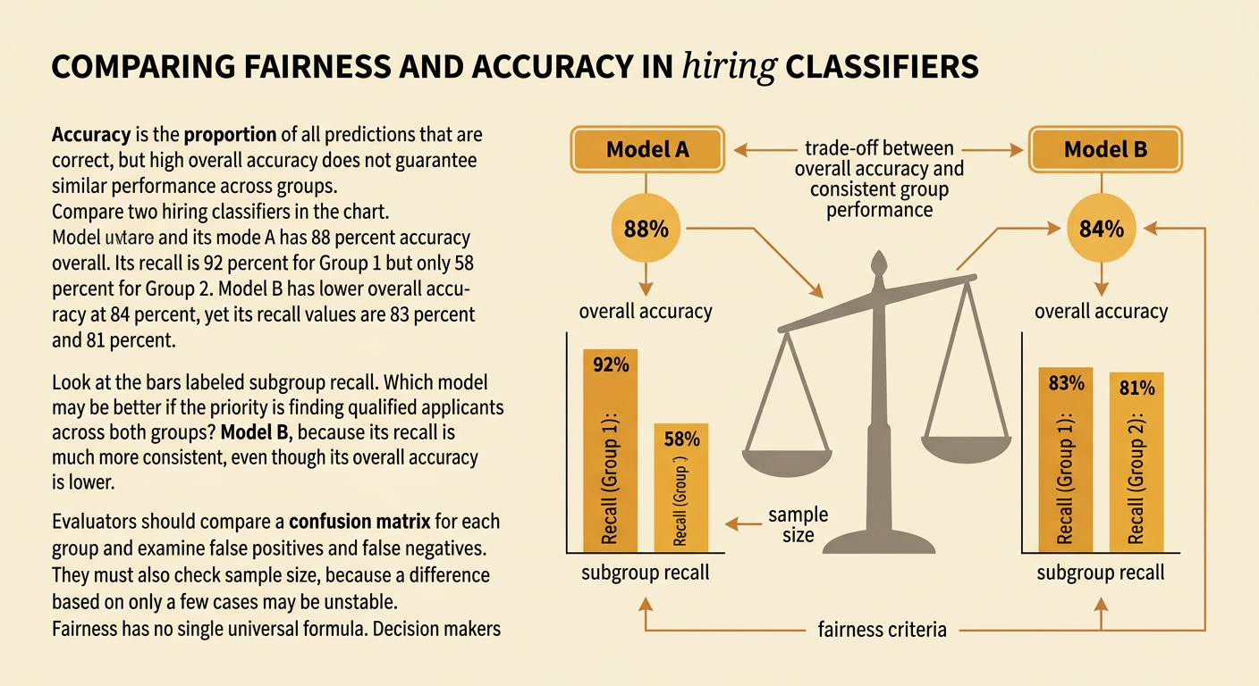
Accuracy measures the proportion of all predictions that are correct, but a highly accurate model can still perform unevenly across groups. Imagine two hiring classifiers. Model A is 88 percent accurate overall, but its recall is 92 percent for Group 1 and 58 percent for Group 2. Model B is 84 percent accurate overall, with recall values of 83 percent and 81 percent for the two groups. If finding qualified applicants across groups is a priority, Model B may be preferred despite its lower overall accuracy. Evaluators should compare subgroup confusion matrices, check whether error-rate differences are supported by adequate sample sizes, and consider the real-world costs of false positives and false negatives. Fairness does not have one universal measure, so decision makers must state their criteria, examine trade-offs, and monitor the deployed model as applicants and conditions change.