
Expected Value and Fair Games
Students calculate and interpret expected values for probability distributions to compare games and evaluate whether their rules are fair.
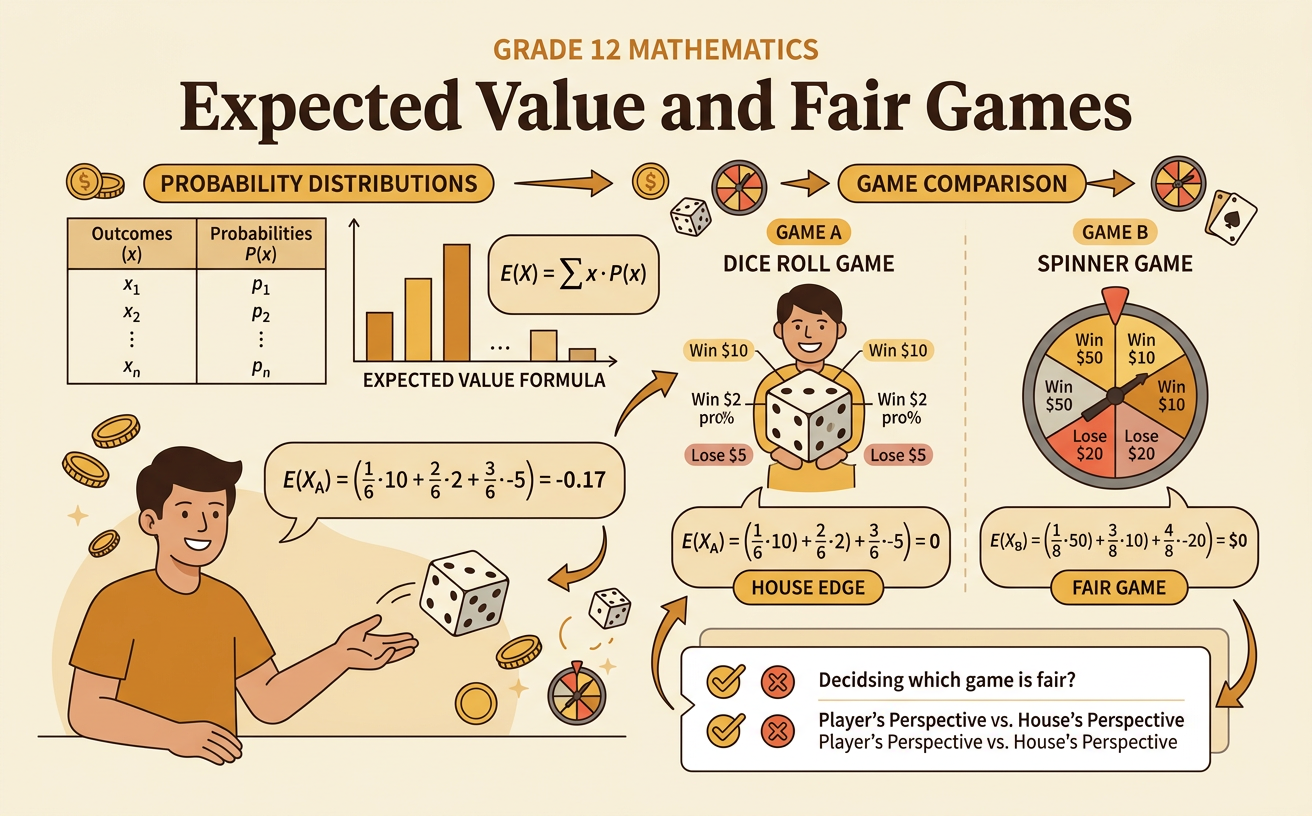
Illustrations are auto-generated and may be placeholders. They can be refreshed to match the narration.
Random Variables and Outcomes
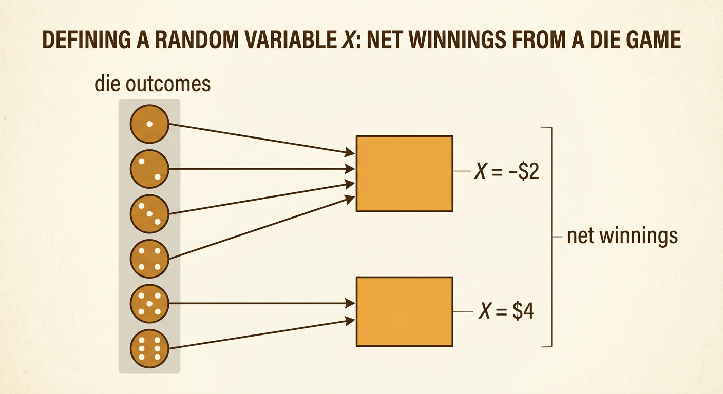
A random variable assigns a numerical value to every outcome of a chance process. The individual outcomes describe what happens, while the random variable records the quantity being studied, such as points, winnings, or waiting time. Suppose a game uses a fair six-sided die. If the result is 1, 2, 3, or 4, the player loses $2. If the result is 5 or 6, the player wins $4. Let X represent the player’s net winnings. Although the die has six possible outcomes, X has only two possible values: −$2 and $4. Outcomes 1 through 4 all map to X = −$2, while outcomes 5 and 6 map to X = $4. Defining the random variable clearly is the first step toward calculating expected value.
Building a Probability Distribution
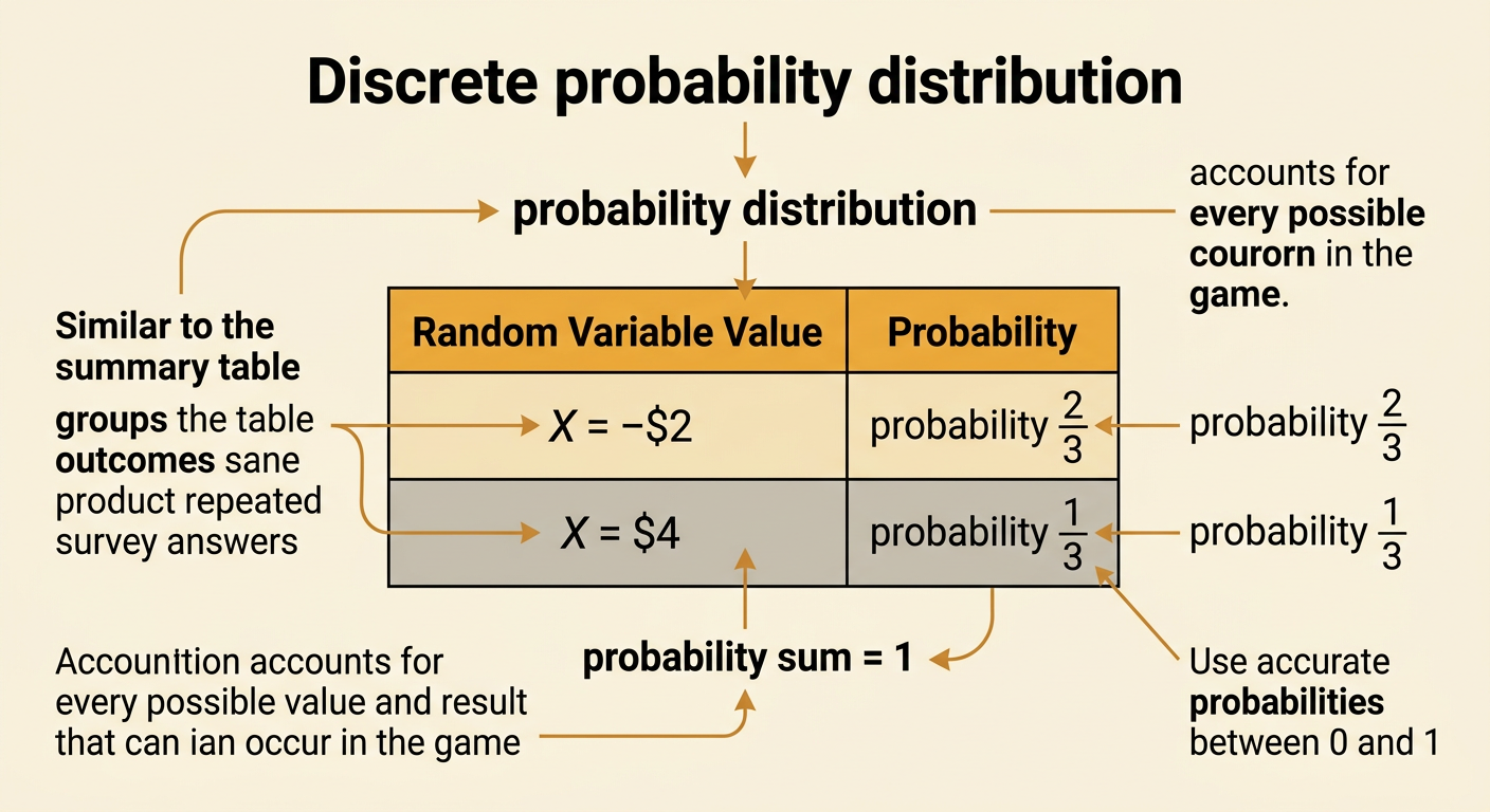
A probability distribution lists every possible value of a random variable and the probability of that value. For the die game, X = −$2 when the die shows 1, 2, 3, or 4. Because four of the six equally likely outcomes cause this result, P(X = −$2) = 4/6 = 2/3. The value X = $4 occurs when the die shows 5 or 6, so P(X = $4) = 2/6 = 1/3. A valid probability distribution includes all possible values, assigns each a probability from 0 to 1, and has probabilities that sum to 1. Here, 2/3 + 1/3 = 1. Combining outcomes that produce the same value makes the distribution easier to use when calculating and interpreting expected value.
Calculating Expected Value
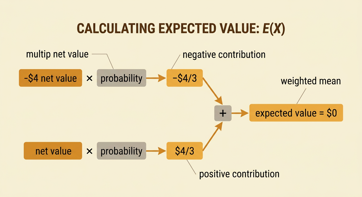
The expected value of a random variable is found by multiplying each possible value by its probability and then adding the products. In symbols, E(X) = ΣxP(X = x). For the die game, E(X) = (−$2)(2/3) + ($4)(1/3). The first product is −$4/3, and the second is $4/3, so E(X) = $0. The negative contribution from the more common loss exactly balances the positive contribution from the less common win. Expected value is a weighted mean because outcomes with greater probabilities have more influence on the result. It is not necessarily one of the possible values: the player can never win exactly $0 on a single play, even though $0 is the expected value.
Interpreting Long-Run Averages
Expected value describes the theoretical average result per trial over many repeated, independent trials. It does not predict the result of one play or guarantee an exact total after a fixed number of plays. In the die game, the expected value is $0 per play. Over 300 plays, about 200 losses and 100 wins would be typical because their probabilities are 2/3 and 1/3. Those approximate counts would produce 200(−$2) + 100($4) = $0. Actual counts may differ, so the total might be positive or negative. As the number of plays becomes very large, the average net winnings per play tend to get closer to $0. This long-run interpretation connects expected value to the mean of the probability distribution.

Comparing Game Fairness
A game is mathematically fair when each side has an expected net gain of $0. The die game is fair by this definition because the player’s expected net winnings are $0. Now compare it with a coin game in which the player wins $3 for heads and loses $2 for tails. For a fair coin, E(X) = ($3)(1/2) + (−$2)(1/2) = $0.50. This game favors the player by an average of $0.50 per play and gives the organizer an expected loss of $0.50. When evaluating a game, use net gains, including entry fees and other costs, rather than advertised prizes alone. Games can have the same expected value but different levels of risk, so expected value determines long-run fairness but does not fully describe the experience of playing.
