
Expected Value of Discrete Random Variables
Students calculate and interpret expected values from discrete probability distributions to compare long-term outcomes in real-world situations.

Illustrations are auto-generated and may be placeholders. They can be refreshed to match the narration.
Define Random Variables
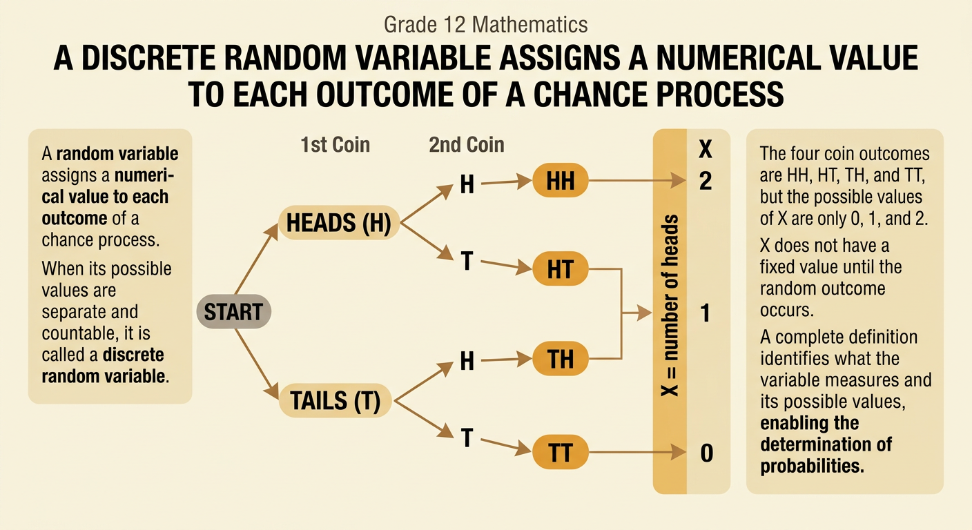
A random variable assigns a numerical value to each possible outcome of a chance process. A discrete random variable has separate, countable values. For example, flip two fair coins and let X represent the number of heads. The possible outcomes are HH, HT, TH, and TT. Therefore, X can equal 0, 1, or 2. If TT occurs, X equals 0; if HT or TH occurs, X equals 1; and if HH occurs, X equals 2. The letter X does not describe one fixed result before the experiment. Instead, its value depends on the random outcome. Clearly defining the variable, including its units and possible values, is the first step toward building a probability distribution and calculating its expected value.
Build a Probability Distribution
A discrete probability distribution lists every possible value of a random variable and the probability of each value. Every probability must be between 0 and 1, and all probabilities must add to 1. Consider a fair spinner divided into four equal sections labeled 0, 2, 2, and 5. Let X be the number of points earned. Although the spinner has four sections, X has only three possible values. The probability that X equals 0 is 1/4, the probability that X equals 2 is 2/4, or 1/2, and the probability that X equals 5 is 1/4. The probabilities total 1. A table or bar graph makes the distribution easy to check and prepares the values for an expected-value calculation.

Calculate Expected Value
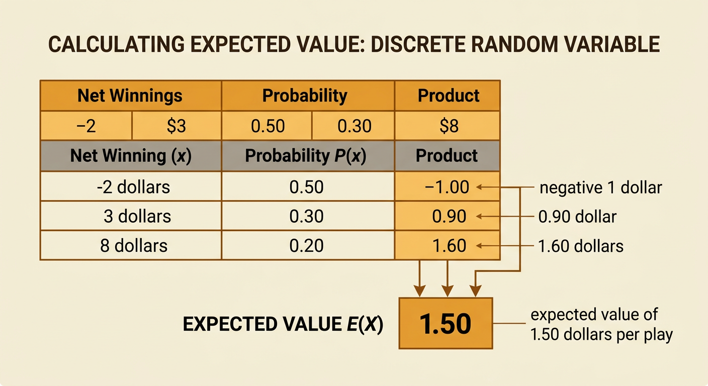
The expected value of a discrete random variable is the mean of its probability distribution. Calculate it by multiplying each possible value by its probability and then adding the products. Suppose a game has net winnings X of negative 2 dollars with probability 0.50, 3 dollars with probability 0.30, and 8 dollars with probability 0.20. The expected value is negative 2 times 0.50, plus 3 times 0.30, plus 8 times 0.20. The products are negative 1 dollar, 0.90 dollar, and 1.60 dollars, so their sum is 1.50 dollars. Thus, the expected value of X is 1.50 dollars per play. The expected value need not be one of the game’s possible individual outcomes.
Interpret Long-Term Outcomes
Expected value describes a long-term average, not a guaranteed result from one trial. In the game with an expected value of 1.50 dollars, no single play pays exactly 1.50 dollars; a player instead loses 2 dollars, wins 3 dollars, or wins 8 dollars. Over many independent plays under the same conditions, the average net winning per play is likely to move closer to 1.50 dollars. For example, after 1,000 plays, the total net winnings might be near 1,500 dollars, although they will rarely equal that amount exactly. Short runs can differ greatly because of random variation. When interpreting expected value, state the variable, its units, and the repeated-trial meaning: in the long run, the mean net winning is about 1.50 dollars per play.

Compare Decision Options
Expected values can compare options by placing their possible outcomes on a common long-term basis. Suppose Option A guarantees a profit of 40 dollars. Its expected value is 40 dollars. Option B gives a profit of 0 dollars with probability 0.50 and 100 dollars with probability 0.50. Its expected value is 0 times 0.50 plus 100 times 0.50, which equals 50 dollars. Option B has the greater expected value, so it produces the larger average profit over many repeated opportunities. However, it also has more variability and can produce no profit on a particular trial. If the decision happens only once, available resources and tolerance for risk may matter. Expected value provides a rational comparison of long-term means, but it does not measure certainty, fairness, or every consequence of a decision.
