Finding Efficient Routes with Graph Algorithms
Students model a transportation network as a weighted graph and trace Dijkstra’s algorithm to determine the shortest route between two locations.

Illustrations are auto-generated and may be placeholders. They can be refreshed to match the narration.
Representing Networks as Weighted Graphs
A transportation network can be modeled as a weighted graph. Locations become points called nodes, and direct connections become lines called edges. Each edge has a weight representing a measurable cost, such as travel time, distance, fuel use, or toll price. Consider a neighborhood with School A, Library B, Station C, Hospital D, and Community Center E. A direct trip from the school to the library takes 4 minutes, while traveling from the school to the station takes 2 minutes. Drawing these locations and connections as a graph removes unnecessary map details while preserving information needed for route planning. This mathematical model supports systematic comparison of routes. It also divides a complex transportation problem into smaller questions: Which locations connect directly, what does each connection cost, and which sequence of connections has the lowest total cost?

Defining Nodes, Edges, and Costs
The three main parts of a weighted graph are nodes, edges, and costs. A node represents a location where a traveler may begin, end, or change direction. An edge represents a direct connection between two nodes. A cost, shown as an edge weight, measures what must be spent to use that connection. In the example network, Station C and Library B are nodes, the line between them is an edge, and its cost is 1 minute. Costs must use a consistent unit to be compared correctly. A model using minutes should not mix a 3-mile distance with a 5-minute travel time unless both are converted into a common measure. The graph may be undirected if travel is possible both ways at the same cost, or directed if one-way streets and different travel times must be represented.
Tracing Dijkstra’s Algorithm
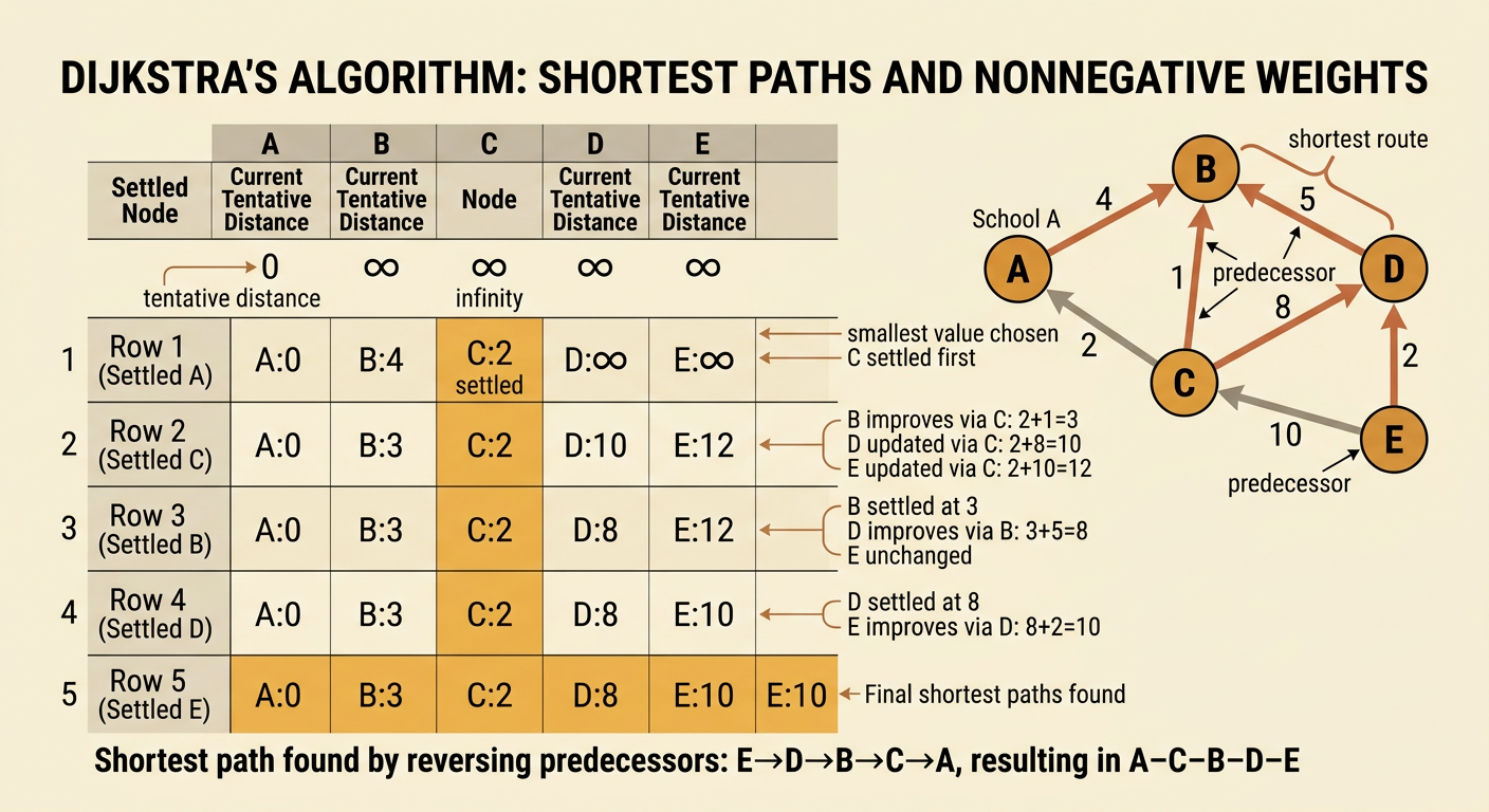
Dijkstra’s algorithm finds the shortest path from one starting node when all edge weights are nonnegative. Begin at School A with a tentative distance of 0; every other node starts at infinity. From A, assign Library B a distance of 4 and Station C a distance of 2. Choose the unsettled node with the smallest distance, C. Through C, B improves to 3 because 2 + 1 = 3; Hospital D becomes 10, and Community Center E becomes 12. Settle B next. Traveling through B improves D to 8 because 3 + 5 = 8, while E remains 12. Settle D and improve E to 10 because 8 + 2 = 10. When E is settled, the shortest distance is final. Following predecessor links backward gives E to D to B to C to A, so the shortest route is A–C–B–D–E.
Comparing Possible Routes
A route’s total cost is the sum of the weights on all edges used. From School A to Community Center E, the route A–C–E costs 2 + 10 = 12 minutes. The route A–B–D–E costs 4 + 5 + 2 = 11 minutes. The route A–C–B–D–E costs 2 + 1 + 5 + 2 = 10 minutes, making it the shortest of these choices. A route with more edges can therefore be faster than a route with fewer edges. Comparing only the number of stops would produce the wrong conclusion. Dijkstra’s algorithm avoids testing every possible route separately by retaining the best known cost to each node. However, route planners should also recognize ties. If two routes have equal minimum costs, either is mathematically shortest, and another criterion, such as reliability or accessibility, may determine the preferred route.

Evaluating Real-World Routing Constraints
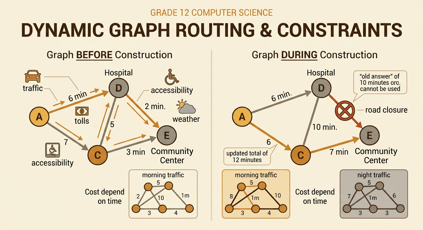
A shortest-path result is only as useful as the model behind it. Real transportation decisions may involve traffic, road closures, tolls, vehicle limits, safety, accessibility, public transit schedules, or changing weather. Suppose construction closes the 2-minute edge from Hospital D to Community Center E. The original 10-minute route becomes unavailable, so the best remaining route from School A is A–C–E, costing 12 minutes. Engineers can manage this change by updating or removing one edge and running the algorithm again. Costs may also vary by time of day, so a graph used during morning traffic could differ from one used at night. Routing technologies can influence where people travel, work, and settle, while population movement can create demand for new roads and transit lines. Evaluating those reciprocal effects connects the mathematical model to engineering design and geographic change.