
Interpreting Linear Models for Energy Use
Students interpret the slope and initial value of a linear energy-use model and use the model to compare the environmental and economic effects of conservation choices.

Illustrations are auto-generated and may be placeholders. They can be refreshed to match the narration.
Review Slope and Initial Value
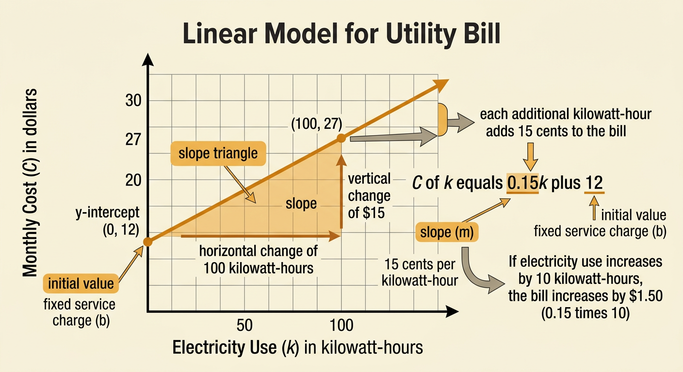
A linear model can be written as y = mx + b. The slope, m, tells how much the output changes when the input increases by one unit. The initial value, b, is the output when the input is zero. Always include units when interpreting these parameters. For example, suppose a utility bill is modeled by C(k) = 0.15k + 12, where k is electricity use in kilowatt-hours and C is the cost in dollars. The slope is $0.15 per kilowatt-hour, so each additional kilowatt-hour adds 15 cents to the bill. The initial value is $12, representing a fixed service charge when no electricity is used. On a graph, the slope controls the line’s steepness, while the initial value is where the line crosses the vertical axis.
Examine an Energy-Use Model
Consider the model E(h) = 1.2h + 6, where h is the number of hours an air conditioner operates each day and E(h) is the home’s total daily electricity use in kilowatt-hours. The model assumes that other household conditions remain similar. If the air conditioner operates for 8 hours, the predicted energy use is E(8) = 1.2(8) + 6 = 15.6 kilowatt-hours. The model’s graph is a straight line because each additional hour adds the same amount of electricity use. A reasonable domain might be 0 through 12 hours per day. Values far outside that domain may not be useful because weather, appliance efficiency, and household behavior can change. A model is a simplified representation, so its predictions should be evaluated using real data when possible.

Interpret Parameters in Context
In E(h) = 1.2h + 6, the slope is 1.2 kilowatt-hours per operating hour. This means each additional hour of air-conditioner use is associated with 1.2 more kilowatt-hours of total daily electricity use. The initial value is 6 kilowatt-hours. It represents the electricity used by lights, refrigerators, electronics, and other household needs when the air conditioner runs for zero hours. For example, increasing air-conditioner use from 5 to 7 hours raises predicted energy use by 1.2(2), or 2.4 kilowatt-hours. The slope describes a marginal effect: the added energy use from one more hour. It does not mean that every appliance uses 1.2 kilowatt-hours per hour. Both parameters must be interpreted using the variables, units, and assumptions of the model.

Compare Conservation Choices
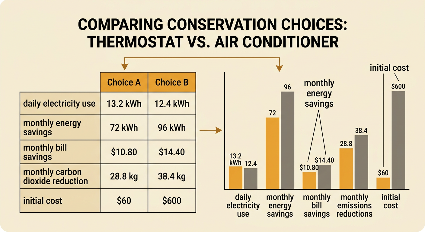
Suppose the home normally runs its air conditioner for 8 hours daily, using 15.6 kilowatt-hours. Choice A is a $60 smart thermostat that reduces operation to 6 hours. The model predicts 13.2 kilowatt-hours daily, a savings of 2.4 kilowatt-hours. Choice B is a $600 efficient air conditioner modeled by E(h) = 0.8h + 6. At 8 hours, it uses 12.4 kilowatt-hours, saving 3.2 kilowatt-hours daily. Over 30 days, the choices save 72 and 96 kilowatt-hours, respectively. At $0.15 per kilowatt-hour, their monthly bill savings are $10.80 and $14.40. If electricity production releases 0.4 kilogram of carbon dioxide per kilowatt-hour, the monthly emissions reductions are 28.8 and 38.4 kilograms. Choice B has the larger environmental benefit, but it also has the larger initial cost.
Justify a Recommendation
A recommendation should balance marginal benefits and marginal costs over a stated time period. Under the given assumptions, the smart thermostat recovers its $60 cost in about 5.6 months because $60 divided by $10.80 per month is approximately 5.6. The efficient air conditioner recovers its $600 cost in about 41.7 months. Over five years, the thermostat saves about 4,320 kilowatt-hours, $648 before its purchase cost, and 1,728 kilograms of carbon dioxide. The efficient unit saves about 5,760 kilowatt-hours, $864 before its purchase cost, and 2,304 kilograms of carbon dioxide. For a household with a limited budget, the thermostat is a strong first choice because it has a short payback period and meaningful environmental benefits. A household prioritizing larger emissions reductions may prefer the efficient unit. The recommendation should be revised if electricity prices, equipment life, or emissions rates change.
