Mapping Environmental Data with Coordinates

Students encode environmental observations as coordinate-based records, plot them as a digital map layer, and use spatial patterns to propose monitoring locations.

Geographic Data as Digital Records

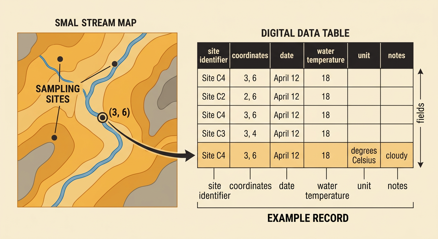
Geographic data connects information to places. In a computer, each observation can be stored as a record, or one row of related values. Useful fields include a site identifier, coordinates, date, measured variable, value, unit, and notes. For example, a student testing Willow Creek might record Site C4, coordinates (3, 6), April 12, water temperature, 18, degrees Celsius, and cloudy water. Consistent records are important because mapping software expects each field to contain the same kind of information. A number without a unit can be misunderstood, and a place name without coordinates may be difficult to map. Digital records can be sorted, compared, updated, and displayed as map symbols. They also preserve evidence so another group can understand where, when, and how an environmental observation was made.

Encode Locations with Coordinates

Coordinates describe a location using an ordered pair, written as (x, y). The x-coordinate tells how far to move horizontally from the origin, and the y-coordinate tells how far to move vertically. Always read x first and y second. Suppose a local park map uses a square grid with its origin at the southwest corner. If a litter survey site is at (4, 2), move four grid squares east and two squares north. Scale converts grid distance to real distance. If one square represents 100 meters, the site is 400 meters east and 200 meters north of the origin. Every record must use the same origin, grid direction, and scale. Otherwise, two groups could enter correct-looking coordinates that refer to different real locations. Coordinates should also match the map boundary and be checked before plotting.

Plot an Environmental Data Layer

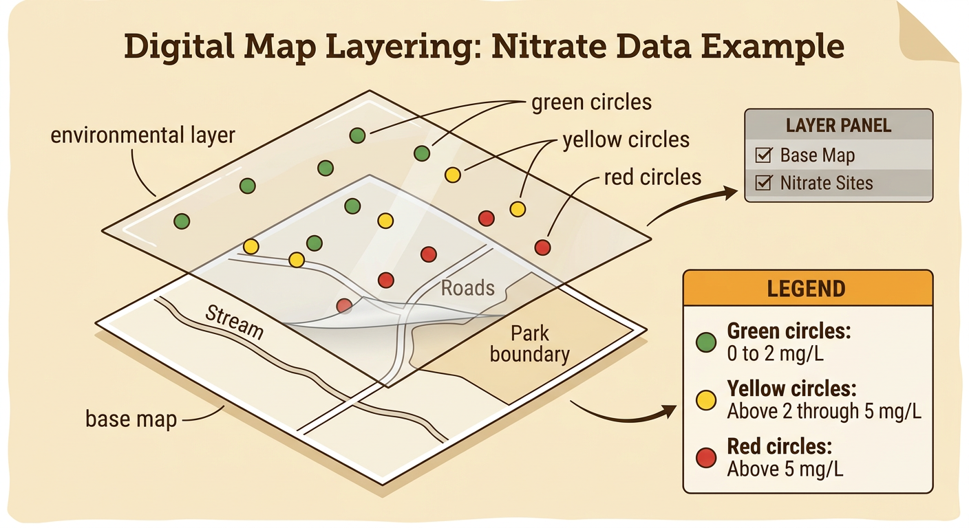
A digital map layer is a group of related features displayed over a base map. The base map might show roads, streams, buildings, and park boundaries. An environmental layer could show air-quality sensors or water-testing sites. To create a layer, mapping software reads each record’s coordinates and places a point at that location. The point can then be styled using the measured value. For example, stream nitrate results might use green circles for 0–2 milligrams per liter, yellow circles for values above 2–5, and red circles for values above 5. A clear legend explains every color. Students should confirm that all points fall in reasonable places and that units are consistent before interpreting the map. Keeping the environmental points on a separate layer also allows users to turn them on or off without changing the base map.

Identify Spatial Patterns

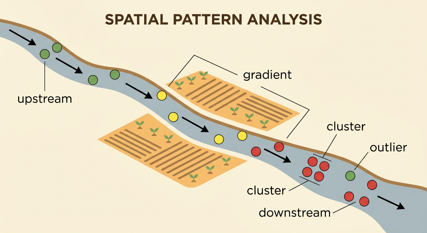
Once points are mapped, look for spatial patterns rather than examining only one value. A cluster is a group of similar observations close together. A gradient is a steady increase or decrease across space. An outlier is a point that differs sharply from nearby points. Imagine that nitrate readings are low upstream, become higher near several fertilized fields, and remain high downstream. This pattern suggests that investigators should study whether runoff from the fields may be entering the stream. However, the map alone does not prove the cause. Rainfall, leaking pipes, or measurement errors could also affect the results. Check dates, units, and unusual records, and compare the layer with roads, land use, drainage, or satellite images. Repeated measurements can show whether the pattern continues or was caused by a short-term event.

Choose Monitoring Locations

A monitoring plan should collect enough evidence to track environmental impact while remaining safe, practical, and minimally disruptive. Select sites that answer a clear question. To investigate possible runoff from a parking lot, place one water-quality station upstream as a comparison site, one beside the storm-drain outlet, and one downstream to detect changes after water passes the outlet. Repeat measurements after similar time intervals and, when relevant, after rainfall. Use the map scale to check spacing. If two downstream sites are three map centimeters apart on a map where one centimeter represents 200 meters, they are 600 meters apart. Also consider safe access, landowner permission, equipment needs, and sensitive habitats. Avoid placing every sensor inside the same cluster because that would leave other areas unrepresented. A strong plan combines comparison sites, suspected impact sites, and locations that reveal change over distance.

Quick Map Check

Before using a map to make a claim, complete a quick accuracy check. First, verify that every record has a site identifier, coordinate pair, value, and unit. Second, confirm that x and y were entered in the correct order and that all points use the same origin and scale. Third, compare plotted points with known features. A stream sample should not appear inside a building unless the coordinates or base map explain why. Fourth, check that the legend matches the symbols and value ranges. Finally, test one distance calculation. On a map where one centimeter equals 250 meters, a measured distance of four centimeters represents 1,000 meters, or one kilometer. If a point or result seems unreasonable, return to the original record instead of moving or deleting it without evidence.