Modeling Disease Spread with Computer Simulations
Students modify parameters in a simple disease-spread simulation, analyze output data, and recommend a public health intervention based on model evidence and limitations.
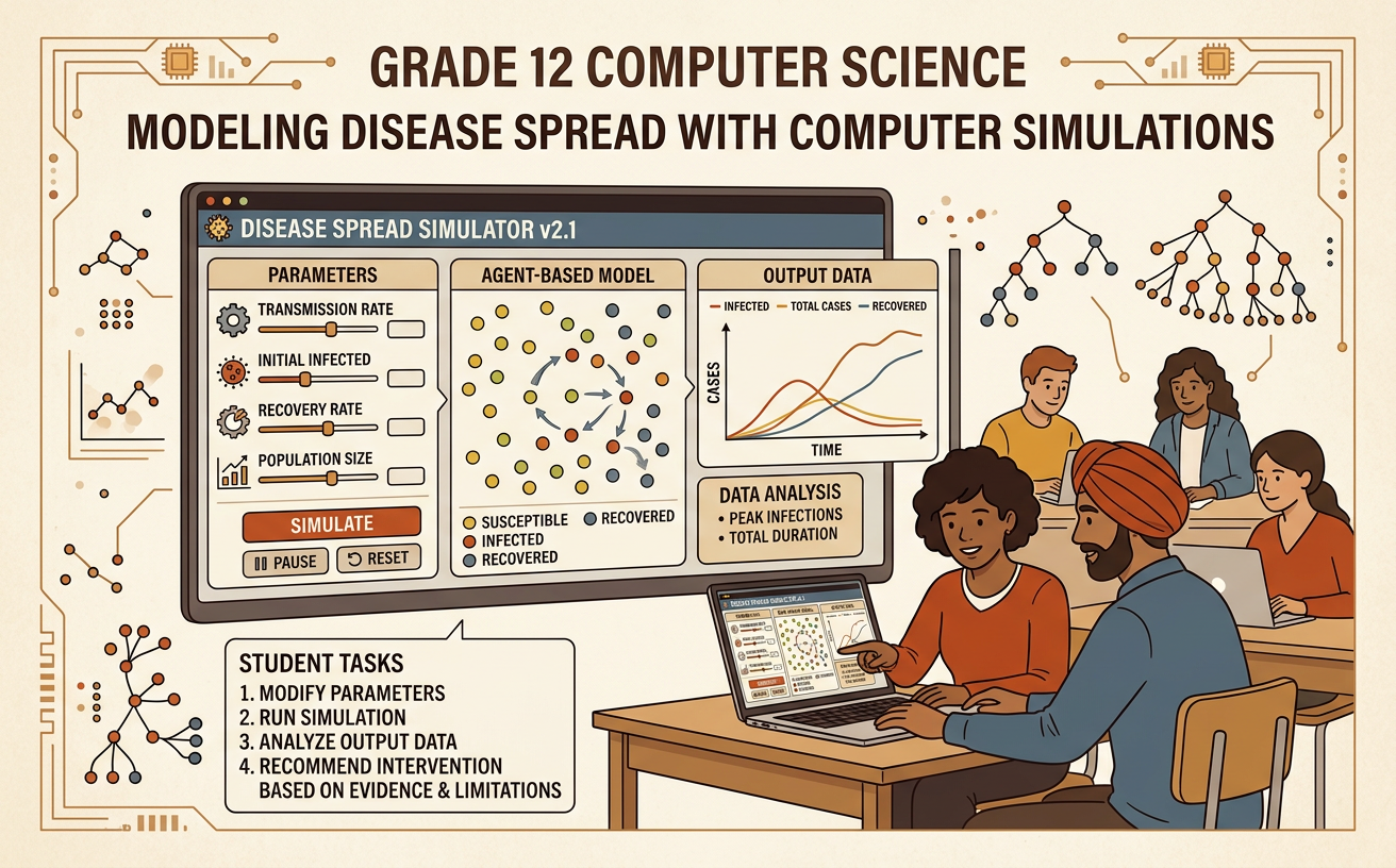
Illustrations are auto-generated and may be placeholders. They can be refreshed to match the narration.
How Computational Simulations Work
A computational simulation uses coded rules to imitate how a system may change over time. In a disease-spread simulation, each person can be represented as susceptible, infected, or recovered. During each simulated day, infected people may contact susceptible people, and each contact has a specified probability of transmission. The program updates everyone’s status and records results such as new infections and total active cases. For example, a model might begin with 1 infected person in a population of 1,000 and simulate 100 days. Because chance affects who becomes infected, repeated runs may produce different outcomes. A simulation does not predict the future with certainty. Instead, it allows researchers to test possible conditions, identify patterns, and compare proposed interventions without exposing real people to disease.

Define Variables and Assumptions
Before running a simulation, identify its variables, fixed values, and assumptions. Input variables are values that users can change, such as population size, initial infections, average contacts per day, transmission probability, infectious period, vaccination rate, or mask use. Output variables are measured results, such as peak active cases, total infections, or the day of the peak. Suppose a model uses 1,000 people, 5 initial infections, 8 contacts per person per day, a 4 percent transmission probability per contact, and a 7-day infectious period. It might assume that everyone mixes randomly and that recovered people cannot be infected again during the simulation. Those assumptions simplify reality and must be stated because they affect the results. Units and allowable ranges should also be defined so that values are interpreted consistently.

Run Baseline and Intervention Scenarios
A baseline scenario represents conditions without the proposed intervention. An intervention scenario changes one or more inputs while keeping other settings the same. This controlled comparison helps connect a parameter change to a difference in output. For example, run a baseline with 8 contacts per person per day and no vaccination. Then test a distancing scenario with 5 contacts per day and a vaccination scenario in which 60 percent of the population begins protected. Run each scenario for the same population and number of days. Because random events can change the outcome, run each scenario many times, such as 100 trials, using different random seeds. Record the median or mean result and the range across trials. Comparing only one run could mistake an unusual outcome for a dependable intervention effect.

Visualize and Compare Output Data
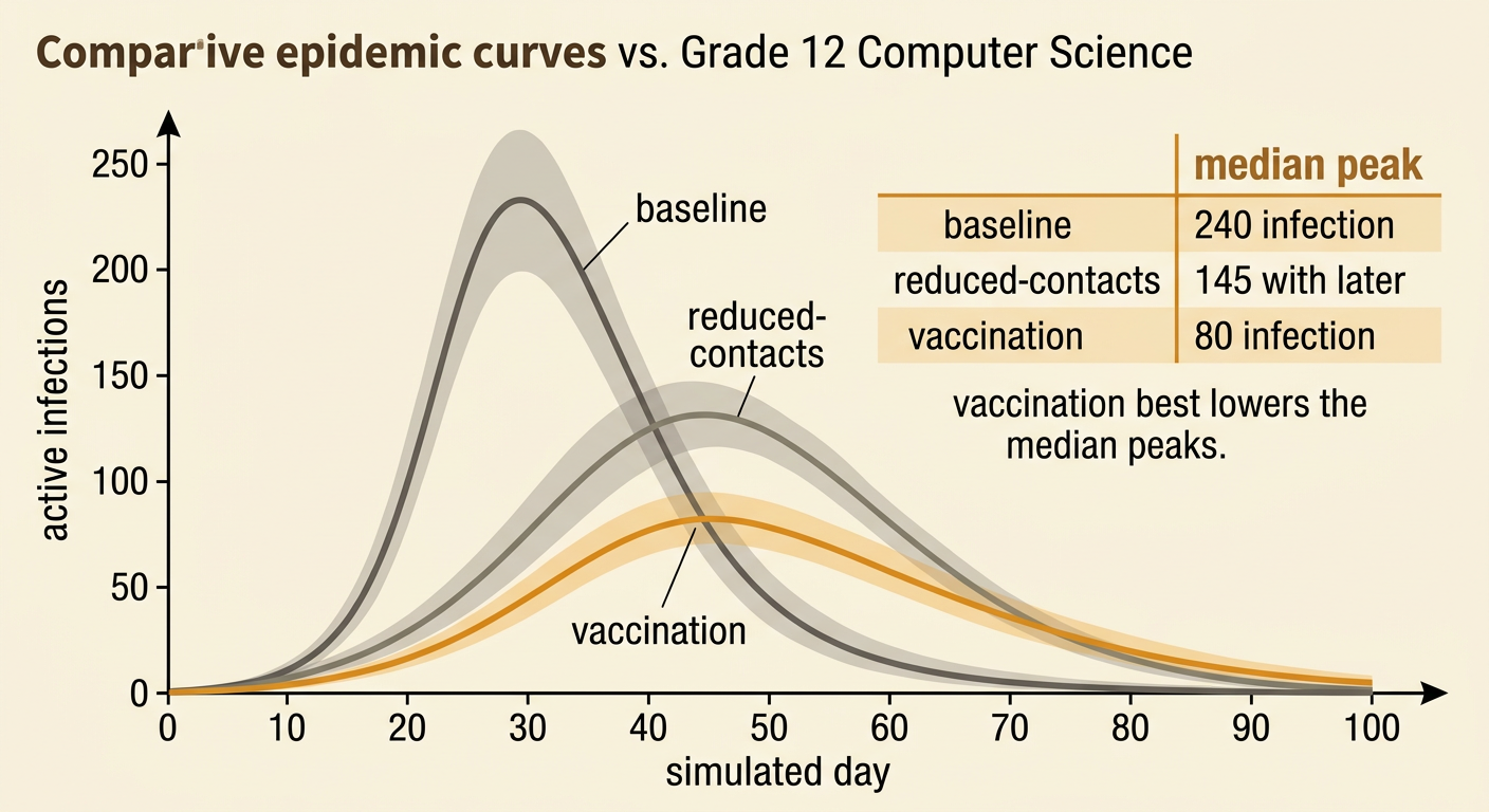
Graphs and summary tables reveal relationships that may be difficult to see in raw output. A line graph can place simulated day on the horizontal axis and active infections on the vertical axis. Separate lines can represent the baseline and each intervention. Compare the height and timing of each peak, the duration of the outbreak, and the area suggested by the curve. A scatterplot can show the relationship between vaccination rate and total infections, with a trend line or curve summarizing the pattern. For example, median peak infections might be 240 in the baseline, 145 with reduced contacts, and 80 with vaccination. Include results from repeated trials by adding shaded intervals or error bars. Always label axes, units, scenarios, and summary statistics so readers can evaluate the evidence accurately.
Evaluate Model Limitations
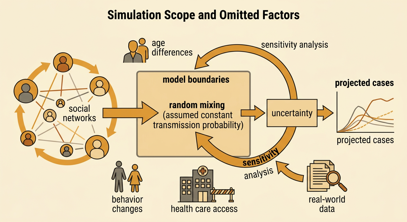
Every simulation leaves out parts of reality, so its results must be interpreted cautiously. A random-mixing assumption ignores the fact that people interact in households, schools, workplaces, and social networks. A constant transmission probability may overlook changing behavior, new variants, seasonality, and differences among individuals. The model may also lack age groups, hospitalization capacity, unequal access to health care, or imperfect compliance with a policy. For example, a scenario that reduces everyone’s contacts from 8 to 5 per day may overestimate the effect if many essential workers cannot reduce their contacts. Test sensitivity by changing uncertain values across plausible ranges and checking whether the main conclusion remains stable. Also compare model outputs with credible real-world data when available. A model is most useful when its assumptions, uncertainty, and boundaries are reported alongside its findings.
Recommend an Evidence-Based Intervention
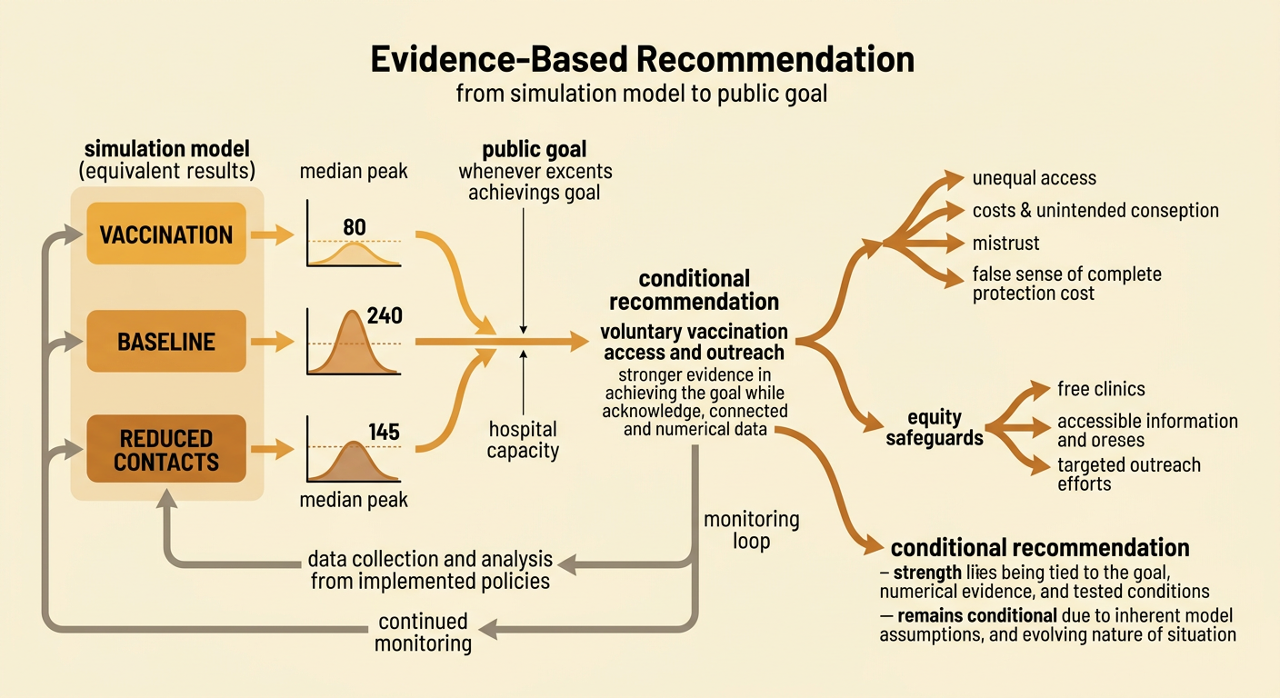
A recommendation should connect simulation evidence to a public goal while acknowledging trade-offs and uncertainty. Begin by identify the outcome being prioritized, such as reducing peak infections to avoid exceeding hospital capacity. Then cite comparable scenario results, explain why the preferred intervention performed better, and describe limitations that could affect the conclusion. For example, if vaccination produced a median peak of 80 active infections compared with 240 in the baseline and 145 under reduced contacts, recommend improving voluntary vaccination access and outreach. Evaluate intended outcomes, such as fewer infections and hospitalizations, as well as possible unintended outcomes, such as unequal access, costs, mistrust, or a false sense of complete protection. Suggest safeguards, including free clinics, accessible information, and continued monitoring. The final recommendation should be conditional: decision-makers should revise the policy if new data or model tests change the evidence.