Modeling Linear Relationships from Tables and Graphs
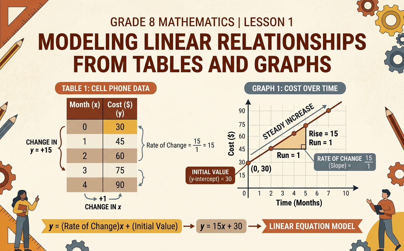
Students identify the rate of change and initial value in tables and graphs, then write linear equations that model the relationships.
Illustrations are auto-generated and may be placeholders. They can be refreshed to match the narration.
Reviewing Linear Relationships
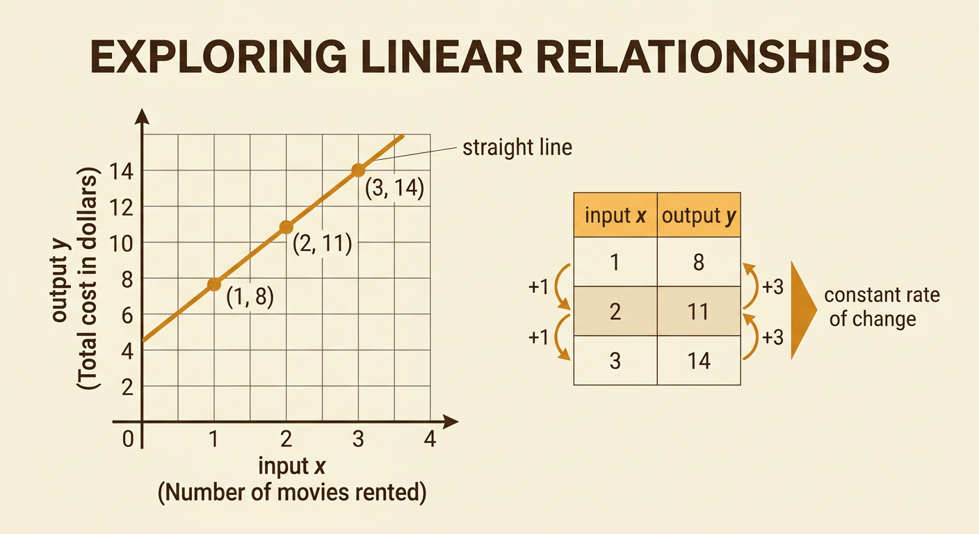
A linear relationship has a constant rate of change. This means that whenever the input changes by the same amount, the output changes by the same amount. In a table, look for a repeated pattern in the differences between values. On a graph, a linear relationship appears as a straight line. For example, suppose a streaming service charges $3 for each movie rented plus a fixed fee. A table includes the points (1, 8), (2, 11), and (3, 14), where x is the number of movies and y is the total cost in dollars. Each time x increases by 1, y increases by 3. Because this change is constant, the relationship is linear. The ordered pairs also lie on one straight line when graphed.
Finding the Rate of Change
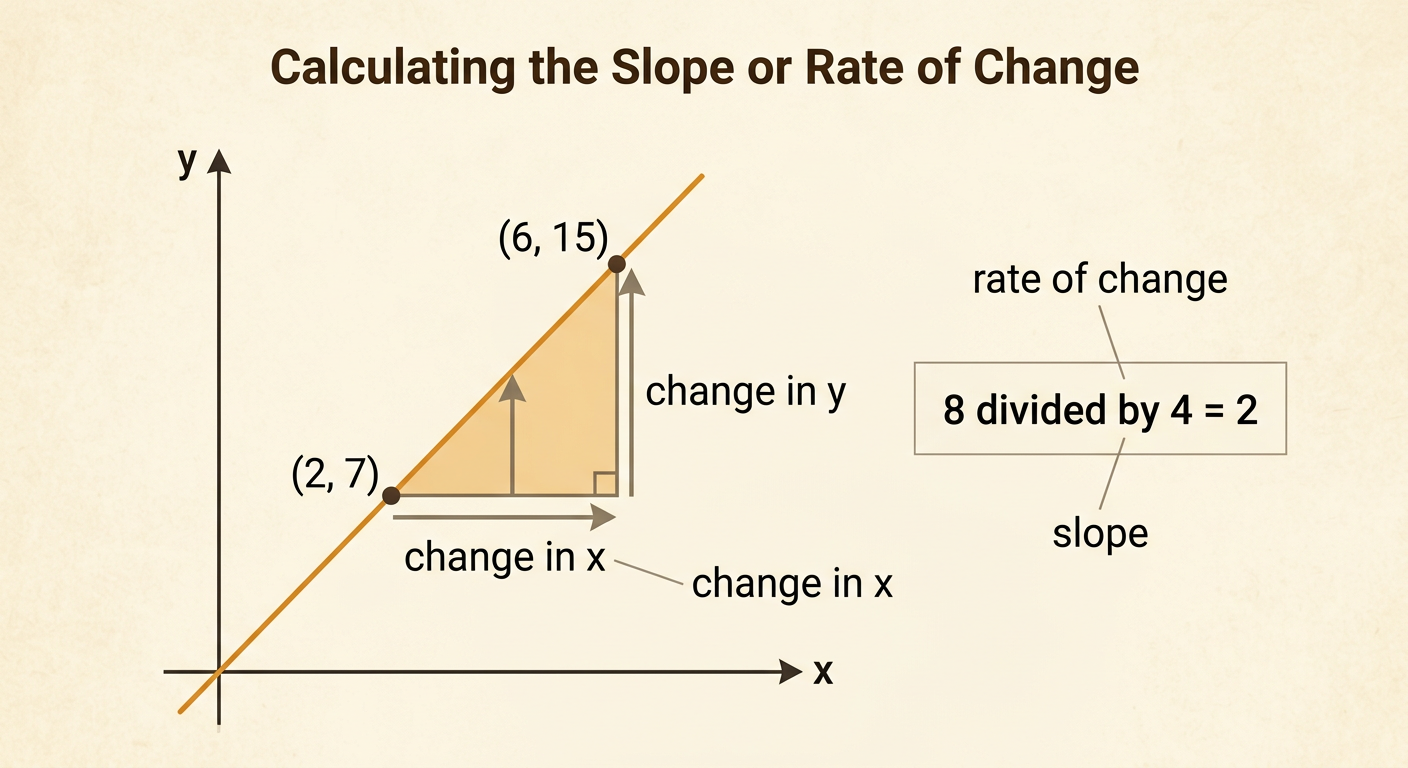
The rate of change tells how much the output changes for each unit of change in the input. It is also called the slope. To find it using two points, divide the change in y by the change in x: rate of change equals (y2 − y1) divided by (x2 − x1). Consider the points (2, 7) and (6, 15). The change in y is 15 − 7, or 8. The change in x is 6 − 2, or 4. The rate of change is 8 divided by 4, which equals 2. This means y increases by 2 whenever x increases by 1. On a graph, this can be shown by moving 4 units to the right and 8 units up from the first point to the second point.
Identifying the Initial Value
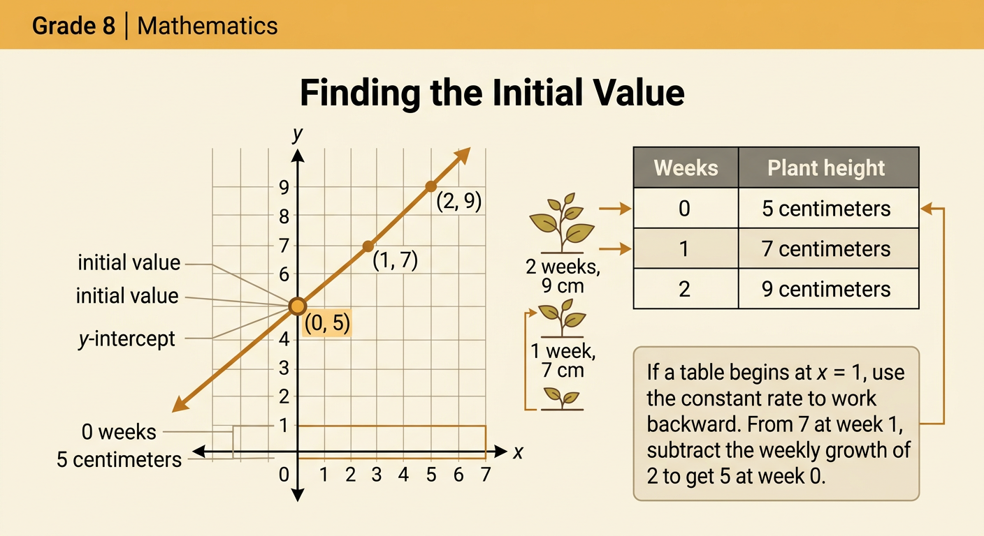
The initial value is the output when the input is 0. In the equation y = mx + b, the initial value is b. On a graph, it is the y-coordinate where the line crosses the y-axis, so it is also called the y-intercept. Suppose a plant is 5 centimeters tall when it is first measured and grows 2 centimeters each week. The point (0, 5) represents the initial measurement because 0 weeks have passed and the height is 5 centimeters. A table might show (0, 5), (1, 7), and (2, 9). The initial value is 5. If a table does not include x = 0, use the constant rate of change to work backward until you determine the output associated with an input of 0.
Writing a Linear Model
A linear relationship can be modeled with the equation y = mx + b. The variable m represents the rate of change, and b represents the initial value. First determine both values from the table or graph, and then substitute them into the equation. For example, a bicycle rental costs an initial fee of $6 plus $4 for each hour. The rate of change is 4 dollars per hour, so m = 4. The initial value is 6 dollars, so b = 6. The model is y = 4x + 6, where x is the number of hours and y is the total cost. For 3 hours, y = 4(3) + 6 = 18. The ordered pair (3, 18) should appear in the table and on the model’s graph.

Interpreting the Equation in Context
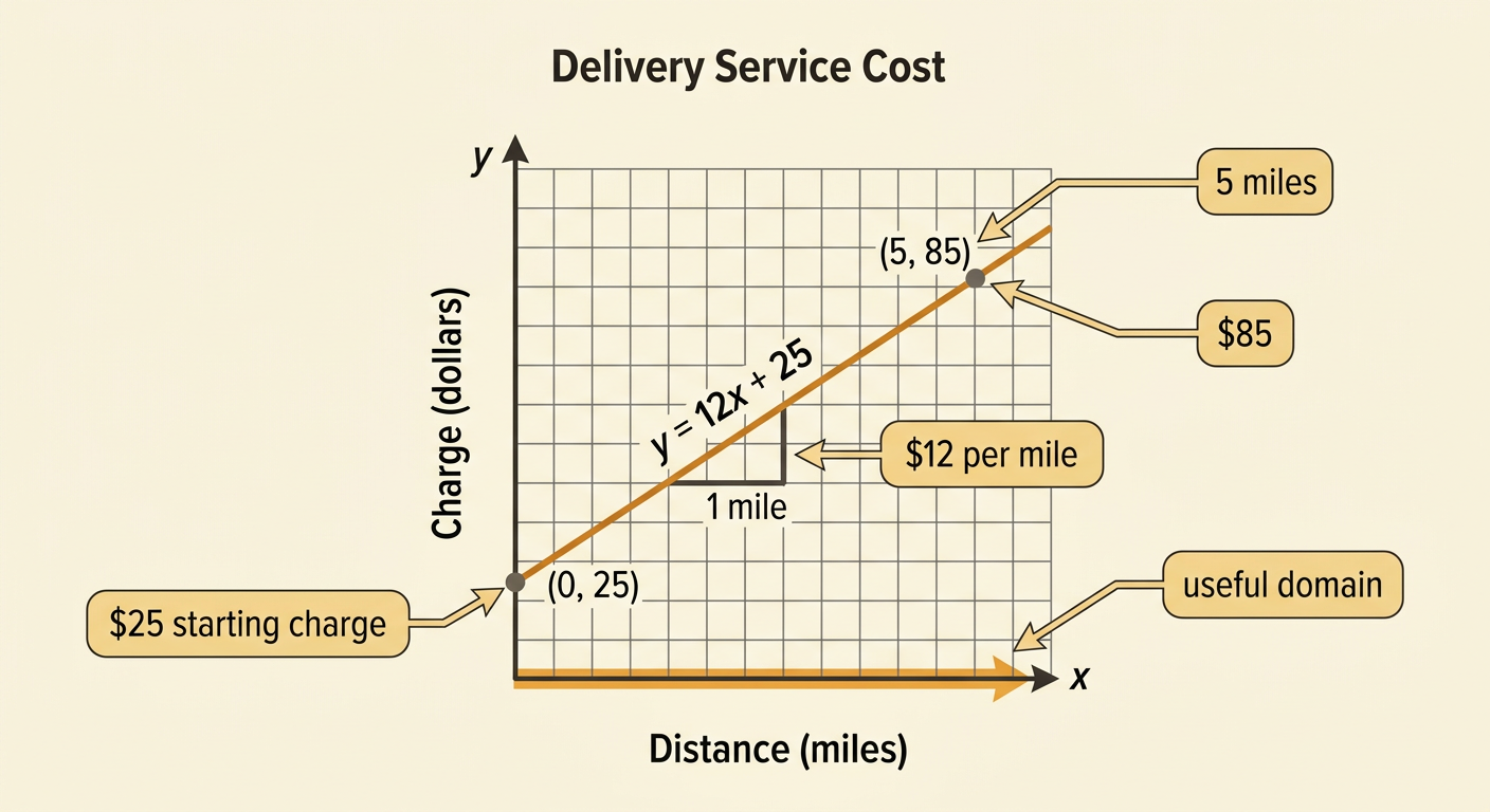
A linear equation is most useful when each number and variable is connected to the situation. Consider y = 12x + 25 for a delivery service, where x is the number of miles and y is the total charge in dollars. The rate of change, 12, means the charge increases by $12 for each additional mile. The initial value, 25, means the service charges $25 even when the distance is 0 miles. To predict the charge for 5 miles, substitute 5 for x: y = 12(5) + 25 = 85. The predicted charge is $85. Always include units when interpreting a model. Also consider reasonable input values. In this situation, negative distances would not make sense, so the useful domain includes only distances of 0 miles or more.