Modeling Radioactive Decay and Half-Life
Students model radioactive decay as an exponential process, calculate remaining isotope quantities, and apply half-life evidence to decisions about nuclear waste management.

Illustrations are auto-generated and may be placeholders. They can be refreshed to match the narration.
Radioactive Isotopes and Nuclear Stability
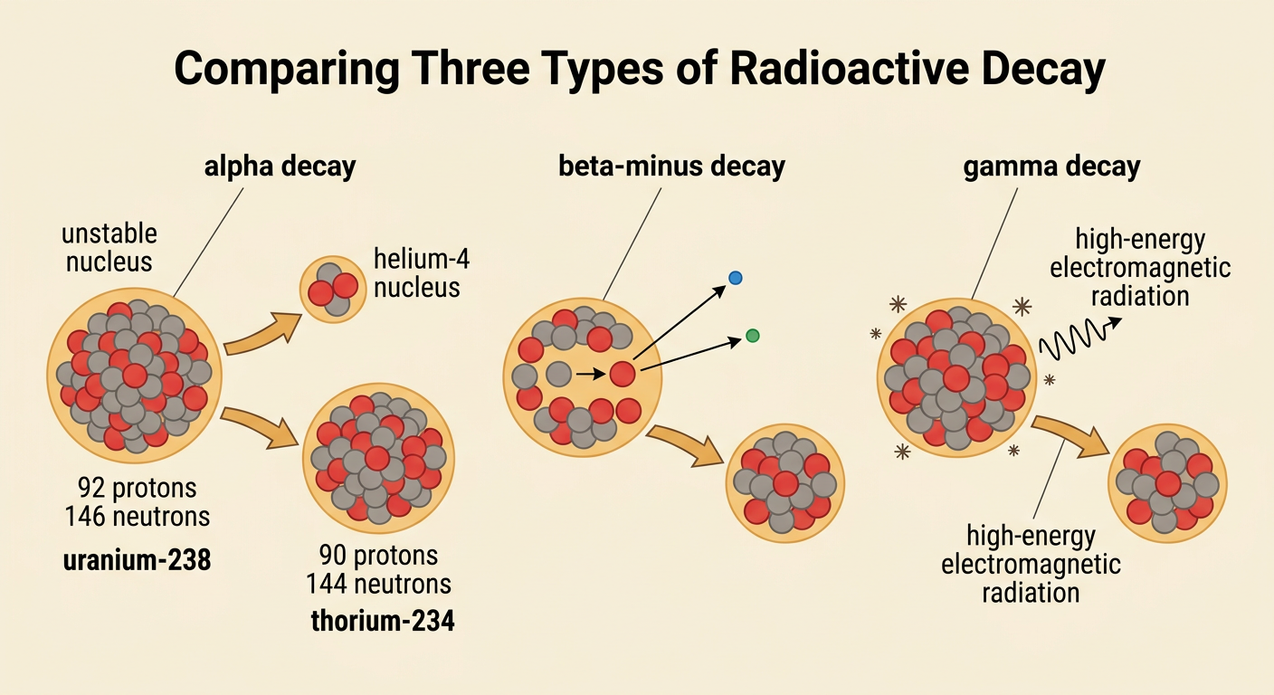
Isotopes are atoms of the same element with the same number of protons but different numbers of neutrons. Some combinations of protons and neutrons make an unstable nucleus. To become more stable, the nucleus can release particles or electromagnetic energy through radioactive decay. In alpha decay, the nucleus emits two protons and two neutrons, so it becomes a different element. In beta-minus decay, a neutron changes into a proton while an electron and an antineutrino are emitted. Gamma decay releases high-energy electromagnetic radiation without changing the numbers of protons or neutrons. For example, uranium-238 undergoes alpha decay to form thorium-234. The products have slightly less mass than the original system; that mass difference appears as released energy, consistent with E = mc².
Understanding Half-Life
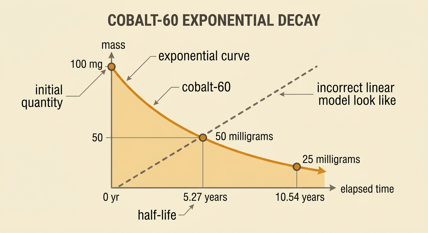
Half-life is the time required for half the radioactive nuclei in a sample to decay. It is a statistical property of a large collection of nuclei, not a timer for one particular atom. After each half-life, half of the amount present at the beginning of that interval remains. Suppose a 160-gram sample has a half-life of 10 years. After 10 years, 80 grams remain; after 20 years, 40 grams remain; and after 30 years, 20 grams remain. The amount lost is not constant: 80 grams decay during the first interval, but only 40 grams decay during the second. This pattern distinguishes exponential decay from linear change. A linear model would subtract the same mass each interval, while radioactive decay multiplies the remaining mass by the same fraction.

Building an Exponential Decay Model
Radioactive decay can be modeled by N(t) = N₀(1/2)^(t/T), where N₀ is the initial quantity, t is elapsed time, and T is the isotope’s half-life. The ratio t/T gives the number of half-life intervals. Because the remaining amount is repeatedly multiplied by 1/2, the model is exponential rather than linear. For cobalt-60, whose half-life is about 5.27 years, a 100-milligram sample can be modeled as N(t) = 100(1/2)^(t/5.27). After 5.27 years, the model gives 50 milligrams; after 10.54 years, it gives 25 milligrams. The smooth curve also estimates amounts between complete half-lives. Although the quantity approaches zero mathematically, the model does not predict that every radioactive nucleus disappears at a specific finite time.
Calculating Remaining Isotope Quantities
To calculate a remaining quantity, identify the initial amount, elapsed time, and half-life, then substitute them into the exponential model. Iodine-131 has a half-life of about 8 days. If a sample begins with 80 milligrams and 24 days pass, the number of half-lives is 24 ÷ 8 = 3. The remaining amount is 80(1/2)³, or 10 milligrams. A table gives the same result: 80 milligrams becomes 40 after 8 days, 20 after 16 days, and 10 after 24 days. For times that are not whole multiples of the half-life, use the exponent t/T without rounding it. The calculated amount describes the expected quantity in a large sample; random decay can cause small measured samples to differ from the exact model.

Evaluating Nuclear Waste Timescales
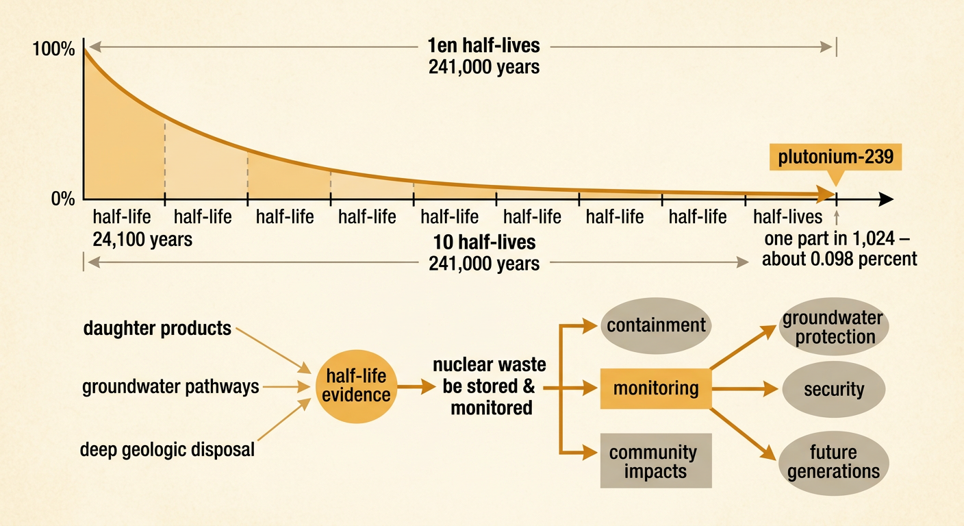
Half-life evidence helps communities evaluate policies for storing and monitoring nuclear waste. Plutonium-239 has a half-life of about 24,100 years. After ten half-lives, or about 241,000 years, the fraction remaining is (1/2)¹⁰ = 1/1,024, which is about 0.098 percent. A small fraction can still matter when the original quantity is large or highly hazardous. Policymakers therefore consider more than half-life: they also examine radiation type, chemical mobility, daughter products, container durability, groundwater pathways, security, cost, and effects on future generations. Deep geologic disposal is intended to isolate waste for very long periods, but possible unintended outcomes include leaks, unequal local burdens, monitoring failures, and loss of institutional knowledge. A strong policy evaluation compares alternatives using scientific evidence while clearly identifying uncertainties, benefits, risks, and who bears the consequences.