
Optimizing Traffic Signals with a Computer Simulation
Students adjust traffic-signal timing in a simple simulation, collect wait-time data, and use the results to recommend an improvement while recognizing the model’s limitations.
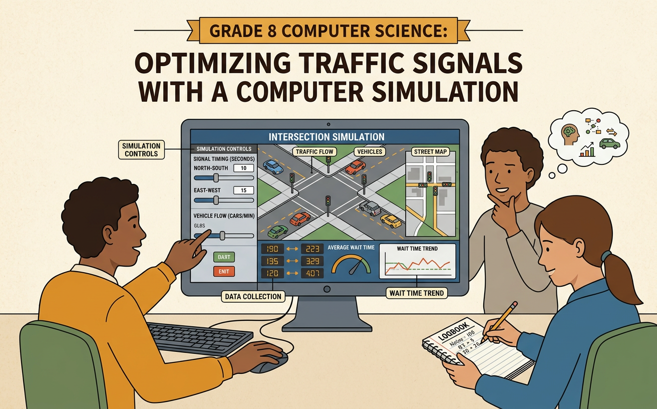
Illustrations are auto-generated and may be placeholders. They can be refreshed to match the narration.
Identify Simulation Inputs and Outputs
A traffic simulation is a computer model of vehicles moving through an intersection. Inputs are values that users or the program provide. They can include green-light duration, vehicle arrival rate, turning percentage, speed, and number of lanes. Outputs are measurements produced by the simulation, such as average wait time, longest wait, queue length, and number of vehicles served. Before testing, identify which inputs will stay constant and which input will change. For example, a model might use 12 east-west arrivals per minute, 8 north-south arrivals per minute, and 30-second green lights in both directions. The output could show an average wait of 40 seconds per vehicle. Clearly separating inputs from outputs helps you design a fair test and understand which change may have caused a result.

Run the Baseline Traffic Model
The baseline is the starting version of the simulation. It gives you data to compare with later tests. Set the initial signal timing and keep all other conditions recorded. Run the baseline several times because random vehicle arrivals can produce slightly different results. For example, use 30-second green lights in both directions and the same arrival rates for five trials. Suppose the average wait times are 41, 37, 40, 39, and 43 seconds. Their mean is 40 seconds. Also record separate waits for each direction and note any unusually long queues. Save the settings, trial results, and run length in a data table. A baseline based on repeated trials is more dependable than a single run and makes later comparisons more meaningful.

Change One Timing Variable
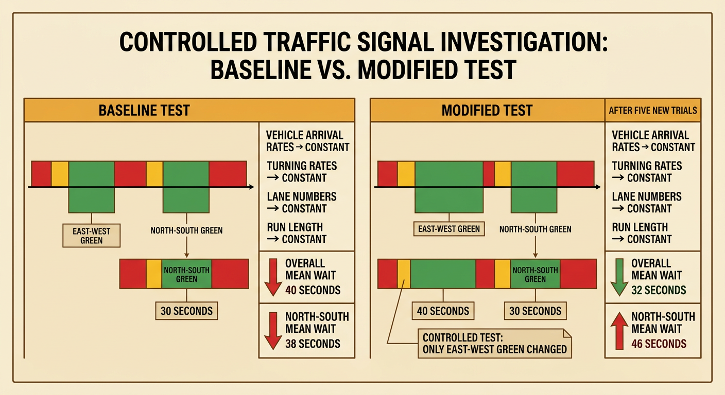
To test cause and effect, change only one timing variable at a time. Keep vehicle arrival rates, turning rates, lane numbers, run length, and other settings the same. For example, increase the east-west green light from 30 seconds to 40 seconds while leaving the north-south green light at 30 seconds. Run five new trials under the same traffic conditions. The new overall mean wait might fall from 40 seconds to 32 seconds. However, the north-south mean wait might rise from 38 seconds to 46 seconds. This shows why you should examine both the total result and the results for different road users. If several variables change together, you cannot tell which change produced the difference. Controlled testing supports careful, iterative improvement of the signal plan.
Graph and Compare Wait Times
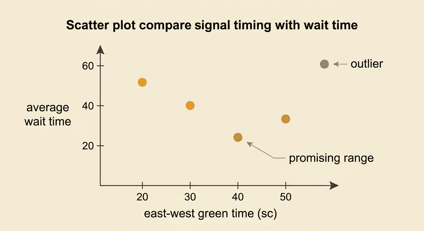
Use a scatter plot to compare signal timing with wait time. Place the timing variable on the horizontal axis and average wait time on the vertical axis. Each point can represent one simulation run. For example, tests with east-west green times of 20, 30, 40, and 50 seconds might produce overall mean waits of 48, 40, 32, and 36 seconds. The points show that wait time decreases at first but rises after 40 seconds. A longer green light can help one direction while forcing the other direction to wait. Look for clusters, trends, gaps, and outliers rather than assuming the relationship is always linear. Compare multiple trials at each timing value, and use the plotted evidence to identify a promising range for further testing.
Recommend a Signal-Timing Policy
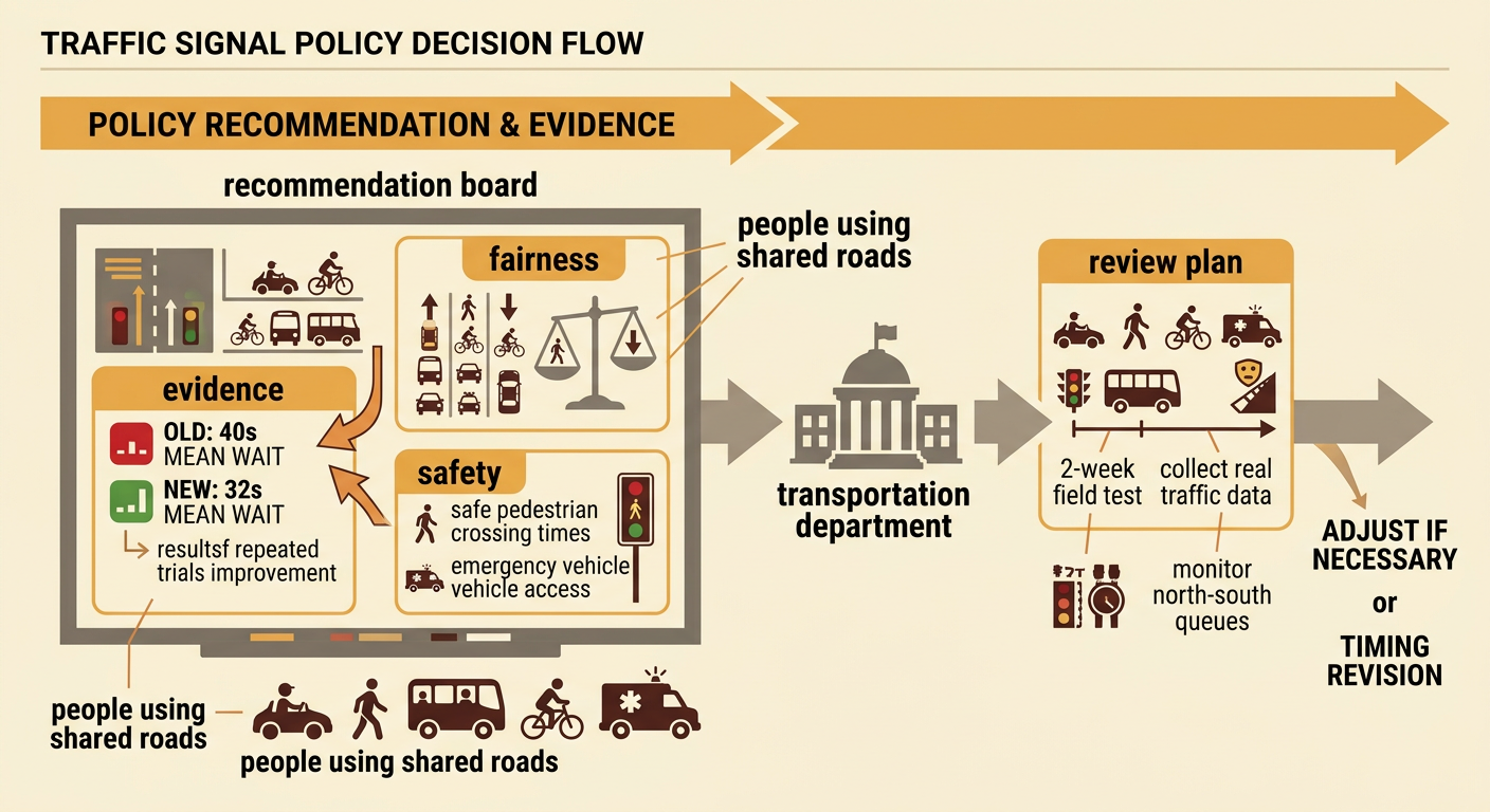
A signal-timing recommendation is a public policy choice because it affects how people use shared roads. Base the recommendation on data, but also consider safety, fairness, cost, and implementation. For example, recommend a 40-second east-west green during the afternoon rush if repeated trials show that it lowers overall mean wait from 40 seconds to 32 seconds. Explain that the city should monitor north-south queues so one group does not receive an unfair burden. The transportation department might first test the plan for two weeks, collect real traffic data, and adjust the timing if needed. Consider consequences for drivers, bus riders, pedestrians, bicyclists, emergency vehicles, and nearby residents. A strong recommendation states the evidence, identifies who will implement it, predicts benefits and trade-offs, and includes a plan for review.
Identify Limitations of the Model
Every simulation simplifies the real world, so its results are evidence rather than a guarantee. A basic traffic model may assume steady arrival rates, normal weather, working signals, and drivers who follow every rule. It may leave out crashes, road construction, school dismissal, special events, emergency vehicles, pedestrians who need extra crossing time, or buses that stop near the intersection. For example, a 40-second east-west green may perform well with 12 arriving vehicles per minute but create long queues when a stadium event raises the rate to 25 vehicles per minute. Randomness and inaccurate input data can also affect results. List these limitations when presenting a recommendation. Improve the model by adding realistic observations, testing peak and off-peak conditions, and comparing simulated results with data collected at the actual intersection.
