Population Growth and Carrying Capacity: Modeling Ecological Limits
Students analyze population data and use mathematical models to explain how resource availability, competition, and environmental change affect carrying capacity.
Illustrations are auto-generated and may be placeholders. They can be refreshed to match the narration.
Defining Carrying Capacity
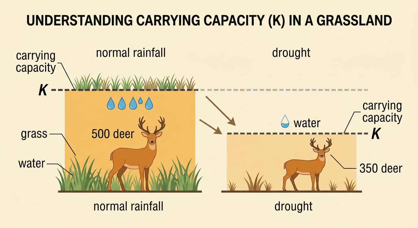
Carrying capacity is the largest population an environment can support over time without exhausting resources or damaging essential habitat. It is usually represented by K. Carrying capacity depends on available food, water, shelter, space, and other conditions, so it is not a permanent or exact number. For example, a grassland might support about 500 deer during years with normal rainfall. A drought could reduce plant growth and lower the carrying capacity to 350 deer. If the population rises above that level, increased competition may reduce survival and reproduction until the population declines. A population can also remain below carrying capacity because of predators, disease, migration, or recent disturbance. Scientists therefore estimate carrying capacity from population trends, resource measurements, and evidence about limiting factors.
Reading Population Growth Graphs
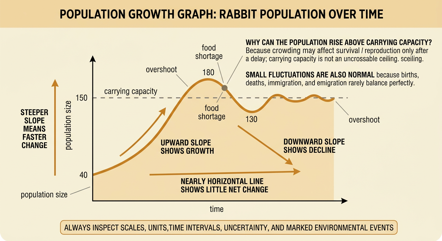
A population growth graph usually places time on the horizontal axis and population size on the vertical axis. An upward slope indicates growth, a downward slope indicates decline, and a nearly horizontal line indicates little net change. The steepness of the slope shows how quickly the population is changing. Small fluctuations around a horizontal carrying-capacity line are common because births, deaths, immigration, and emigration do not balance perfectly. For example, an island rabbit population may rise from 40 to 180, overshoot an estimated carrying capacity of 150, and then fall to 130 after food becomes scarce. That pattern suggests delayed effects of crowding rather than a fixed ceiling that the population cannot cross. When interpreting a graph, examine axis scales, units, time intervals, uncertainty, and any marked environmental events.
Exponential and Logistic Models
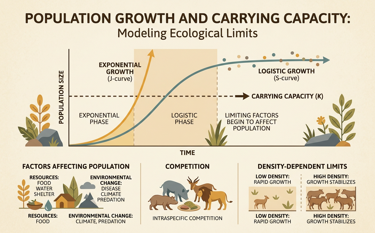
Exponential growth occurs when a population increases by a constant proportion during each time interval and resources are effectively unlimited. It produces a J-shaped curve and can be modeled as dN/dt = rN, where N is population size and r is the per-capita growth rate. Logistic growth includes limits by using dN/dt = rN(1 − N/K). It produces an S-shaped curve: growth begins slowly, accelerates, and then slows as N approaches carrying capacity K. For example, bacteria placed in fresh nutrient broth may grow nearly exponentially at first. As nutrients decline and wastes accumulate, growth slows and the culture approaches a maximum size. Both models are simplifications. Exponential models may describe short periods, while logistic models are more useful when density-dependent limits strengthen as a population becomes crowded.

Limiting Factors and Feedback
A limiting factor is any condition that restricts population growth. Density-dependent factors become stronger as population density increases. They include competition for food or nesting sites, disease transmission, predation, and waste buildup. These factors create negative feedback: population growth increases crowding, crowding lowers survival or reproduction, and slower growth reduces further crowding. Density-independent factors, such as hurricanes, wildfires, freezes, and some human disturbances, can affect populations regardless of density. For example, when a crowded wolf population competes for limited prey, fewer pups may survive, slowing growth. A severe wildfire could reduce the same population even if few wolves were present. Environmental changes can also alter carrying capacity itself. Habitat restoration may raise K, while pollution, drought, or habitat fragmentation may lower it.

Analyzing a Population Dataset
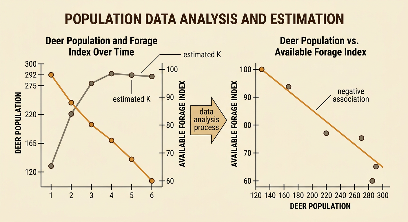
To analyze population data, graph the variables, describe the pattern, and connect the pattern to possible mechanisms. Consider a deer population measured over six years: 120, 165, 220, 275, 292, and 287 deer. Over the same period, available forage measured in index units was 100, 94, 83, 70, 61, and 60. A scatterplot of deer abundance and forage would show a negative association: larger deer populations occur with less available forage. The population’s annual increases also shrink near 290 deer, suggesting a carrying capacity close to that level under the observed conditions. However, correlation does not prove that deer alone caused the forage decline. Rainfall, land use, or measurement error could affect both variables. Scientists should compare trends, calculate changes, inspect outliers, and use additional evidence before choosing a model or estimating K.
Making an Evidence-Based Prediction
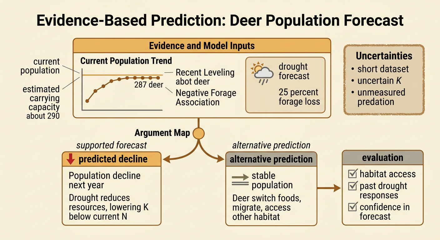
An evidence-based prediction states a claim, supports it with data and a model, and identifies uncertainty. Suppose the deer population is 287, its estimated carrying capacity is about 290, and forecasts predict a drought that will reduce forage by 25 percent. A reasonable claim is that the deer population will decline during the next year because the drought is likely to lower carrying capacity below the current population. Evidence includes the recent leveling of deer numbers and the observed association between high deer abundance and low forage. A competing claim might predict stability because deer could switch foods or migrate. Evaluate both claims by considering habitat access, past drought responses, and confidence in the forage forecast. The final prediction should acknowledge limitations, including the short dataset, uncertain K, unmeasured predation, and possible management actions such as supplemental feeding.