
Reading Climate Data and Forecasting Earth System Impacts
Students interpret temperature, atmospheric carbon dioxide, and sea-level data to explain current climate trends and forecast impacts on Earth systems and human communities.
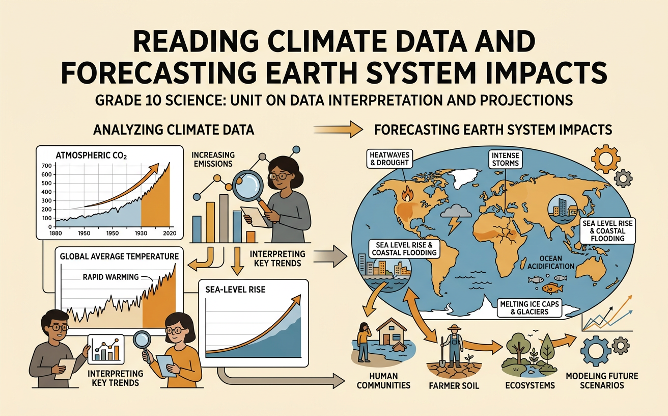
Illustrations are auto-generated and may be placeholders. They can be refreshed to match the narration.
Climate Indicators and Long-Term Trends
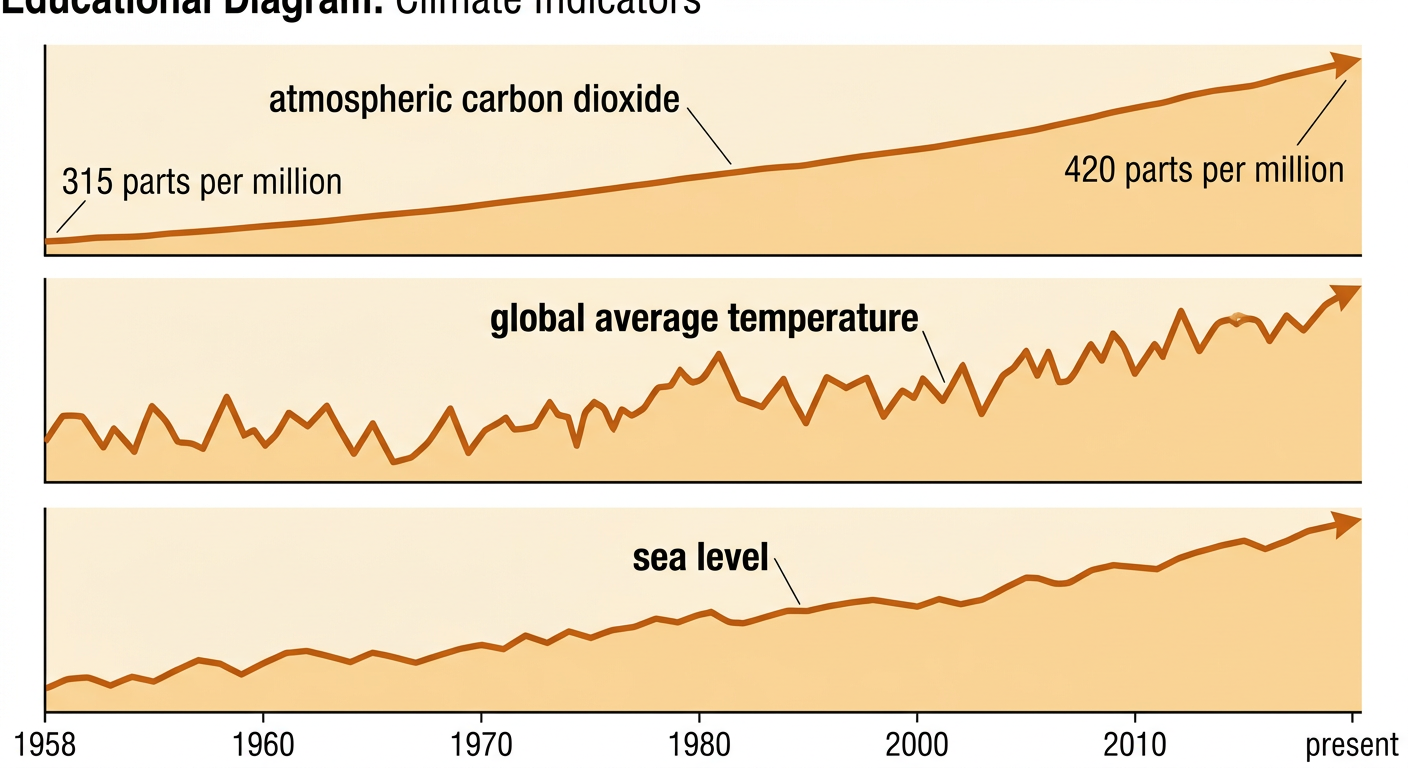
Climate indicators are measurable conditions that reveal how Earth’s climate changes over decades or longer. Important indicators include global average temperature, atmospheric carbon dioxide concentration, sea level, glacier mass, and ocean heat content. A single hot year does not establish a climate trend because weather varies naturally. Scientists instead examine many measurements collected over long periods. For example, carbon dioxide measured at Mauna Loa Observatory increased from about 315 parts per million in 1958 to more than 420 parts per million in recent years. During roughly the same period, global temperature and sea level also rose. Multiple indicators showing related changes provide stronger evidence than one data set alone. Scientists also consider measurement uncertainty, differences among locations, and natural influences such as volcanic eruptions when identifying long-term trends.
Interpreting Graphs and Climate Data
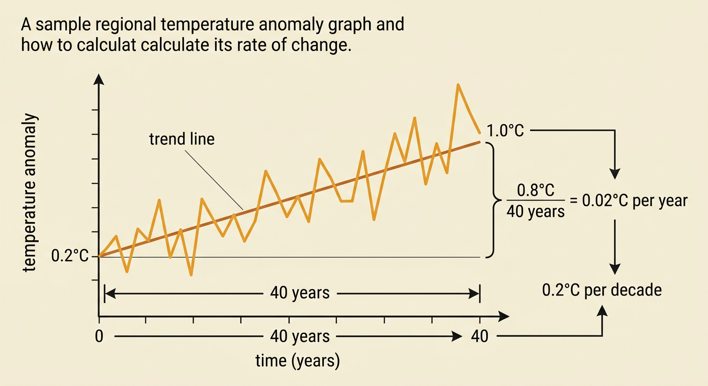
To interpret a climate graph, first read the title, axes, units, time span, scale, and data source. Then identify the overall pattern, short-term variation, and any uncertainty range. A temperature anomaly is the difference between an observed temperature and the average for a reference period; it is not the actual temperature. The rate of change is the change in a value divided by the elapsed time. For example, if a regional temperature anomaly rises from 0.2°C to 1.0°C over 40 years, the average rate is 0.8°C divided by 40 years, or 0.02°C per year. This is also 0.2°C per decade. Translating the graph into a sentence, students could write, “The region warmed overall, although individual years moved above and below the trend line.”
Connections Among Earth Systems
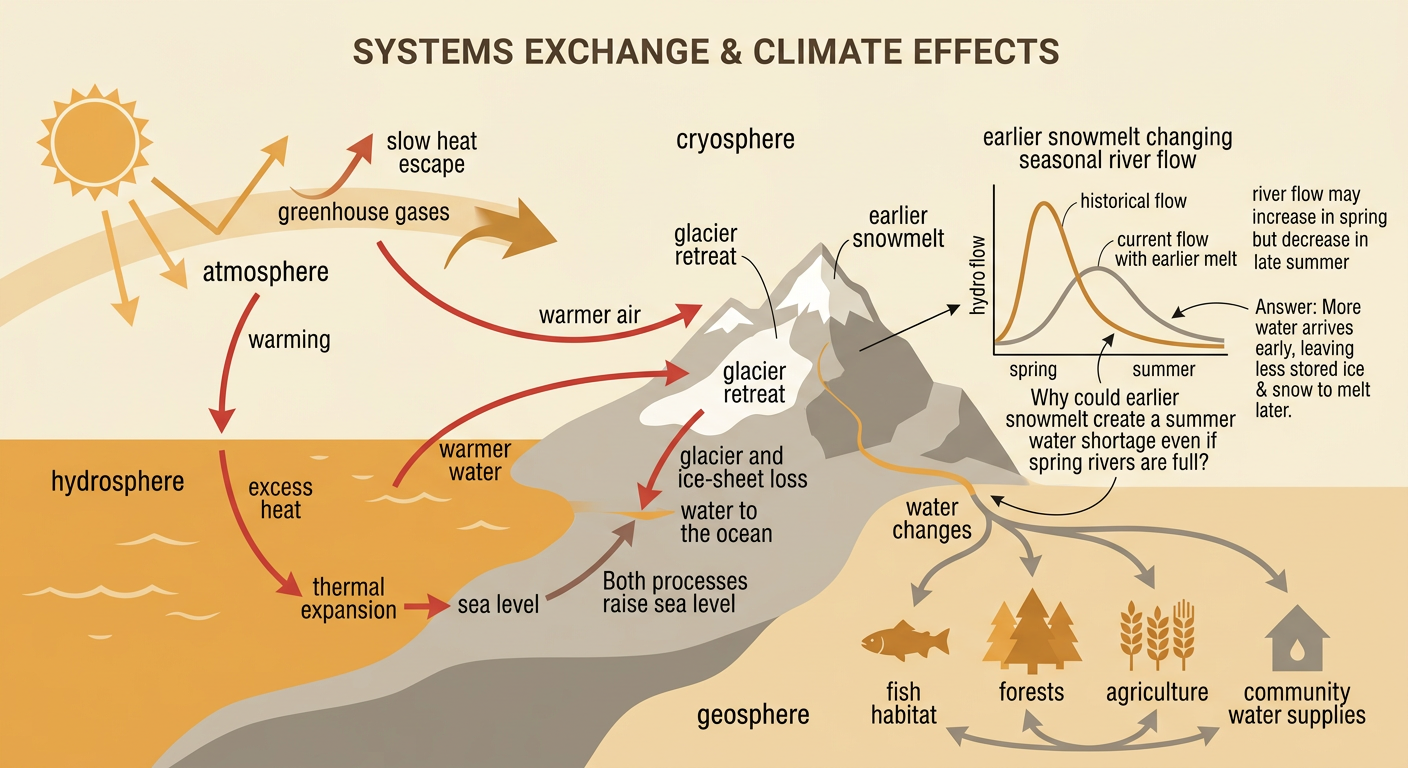
Climate change affects the atmosphere, hydrosphere, cryosphere, geosphere, and biosphere through connected processes. Additional greenhouse gases in the atmosphere reduce the rate at which heat escapes to space. The oceans absorb most of the excess heat added to the climate system, causing seawater to expand. Warmer air and ocean water also contribute to glacier and ice-sheet loss, adding water to the ocean and raising sea level. For example, the retreat of a mountain glacier can reduce cold-season ice storage and change the timing of river flow. Earlier snowmelt may increase spring flow but leave less water available during late summer. These physical changes can affect fish habitat, forests, soils, agriculture, and community water supplies. Because matter and energy move between Earth systems, one climate trend can produce several linked effects.
Forecasting Regional and Global Impacts
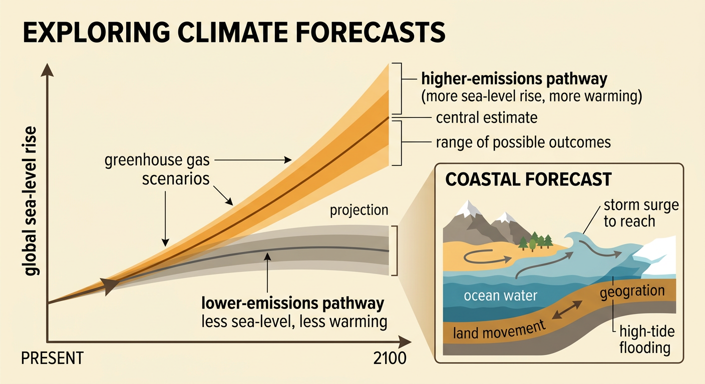
Climate forecasts use observations, physical laws, and computer models to estimate future conditions. Scientists test models by checking whether they reproduce past climate patterns. They then run models under different greenhouse gas scenarios. A projection is conditional: it describes what is likely if a particular scenario occurs. It is not a certain prediction of one exact future. Results from many models can be compared to find the central estimate and range of possible outcomes. For example, a coastal region may combine projected global sea-level rise with local land movement, tides, and storm-surge data. The analysis may show that high-tide flooding will occur more often even when the exact number of events remains uncertain. Regional forecasts can differ from global averages because mountains, ocean currents, vegetation, ice, and local geography influence climate responses.
Effects on Human Communities
Climate trends influence where people live, how they use land, and which resources are available. Effects vary because communities have different exposure, infrastructure, wealth, and ability to adapt. Sea-level rise can damage coastal homes, roads, freshwater supplies, and cultural sites. Increasing heat can raise health risks for outdoor workers and residents without reliable cooling. Shifts in rainfall and snowpack can change farming, hydropower production, and urban water planning. For example, repeated coastal flooding may lead a town to elevate buildings, restore wetlands, restrict new construction, or relocate some residents. Movement caused partly by climate pressures may be temporary or permanent, and it often interacts with jobs, housing costs, conflict, and family connections. Evaluating community impacts therefore requires both climate data and geographic information about population, resources, land use, and vulnerability.

Evidence-Based Climate Explanation
An evidence-based climate explanation includes a clear claim, relevant data, scientific reasoning, and an acknowledgment of uncertainty. The claim answers the question being investigated. Evidence should use specific values, units, dates, rates, or patterns from more than one reliable source. Reasoning explains how the evidence supports the claim through known Earth-system processes. For example, a student might claim that coastal flooding risk will increase. Evidence could include a measured local sea-level trend, projected regional sea-level ranges, and records of past high-tide flooding. The reasoning would explain that a higher average sea level allows tides and storm surges to reach flood thresholds more often. The student should distinguish observations from model projections and describe the projection as a range rather than a guaranteed value. A strong conclusion also identifies limitations, such as uncertain future emissions or local land movement.
