Satellite Orbits and Kepler’s Laws
Students use Kepler’s laws, gravitational relationships, and mathematical models to explain and predict the motion of planets and artificial satellites.

Illustrations are auto-generated and may be placeholders. They can be refreshed to match the narration.
Orbital Motion in Space
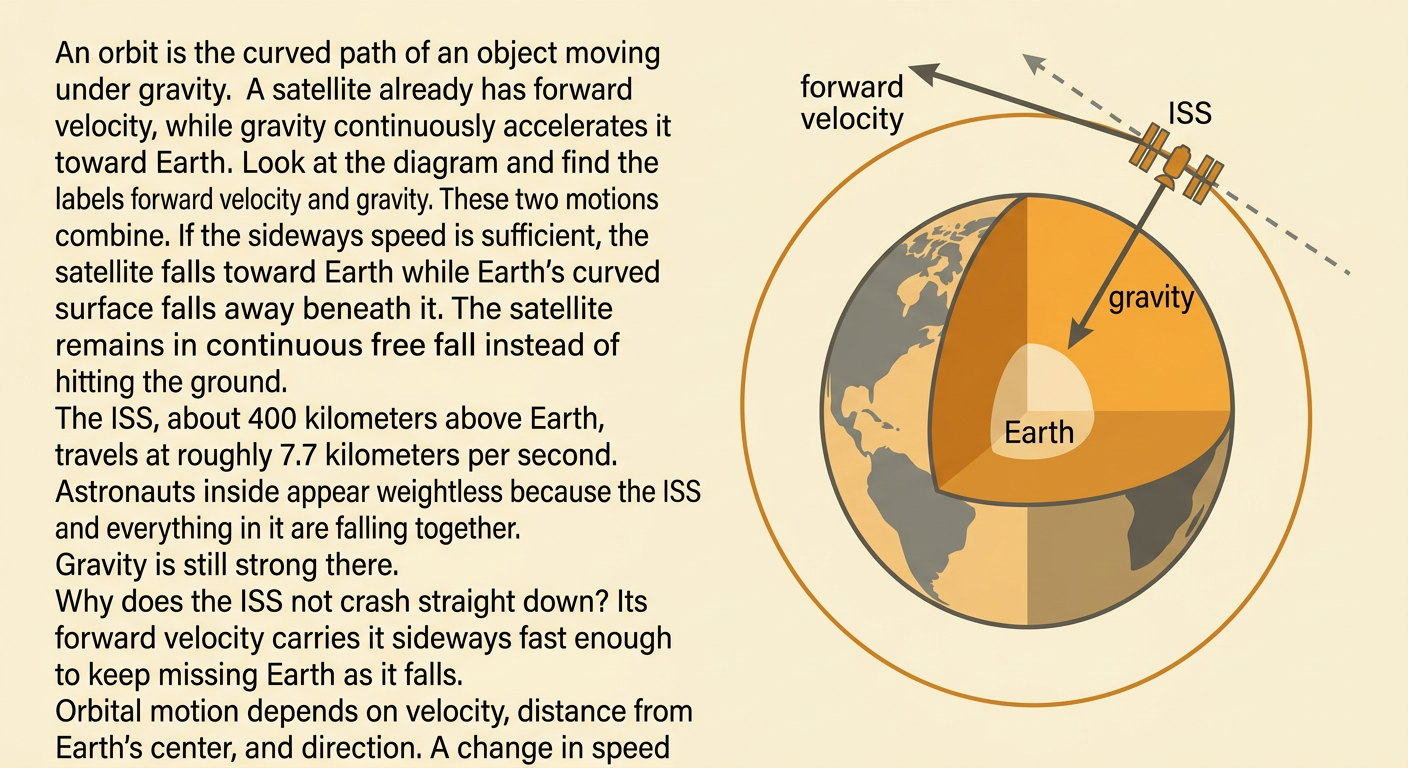
An orbit is the curved path of an object moving under gravity. A satellite has forward velocity, but gravity continuously accelerates it toward the body it orbits. If its sideways speed is sufficient, the satellite keeps falling toward Earth while Earth’s curved surface falls away beneath it. The result is continuous free fall rather than a collision. Orbital motion depends on the satellite’s velocity, distance from Earth’s center, and the direction of motion. For example, the International Space Station travels at about 7.7 kilometers per second while orbiting roughly 400 kilometers above Earth. Astronauts appear weightless because they and the station are falling together, not because gravity is absent. Changing a satellite’s speed or direction changes the size, shape, or orientation of its orbit.
Kepler’s Three Laws
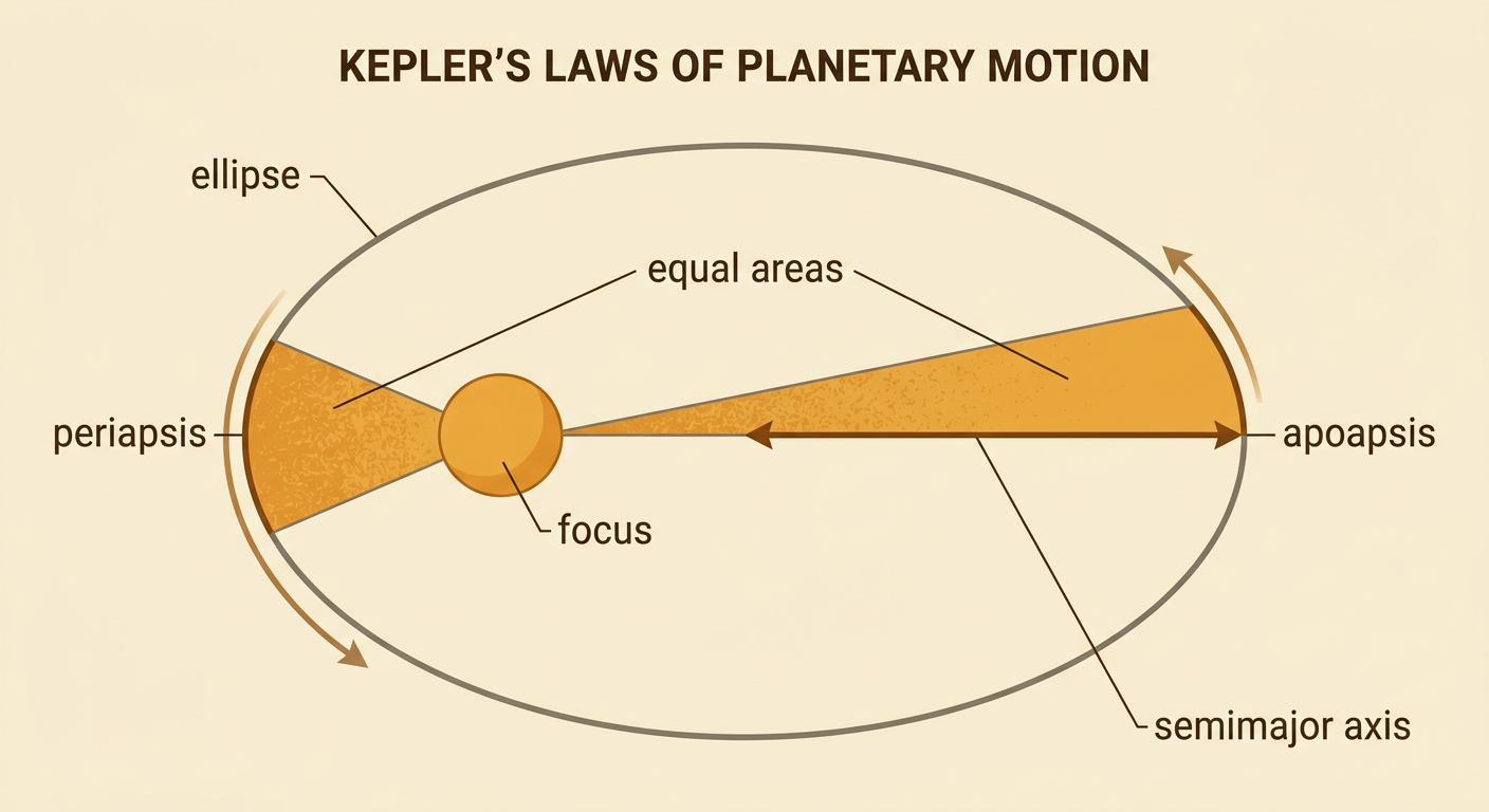
Kepler’s first law states that an orbit is an ellipse with the central body at one focus. A circle is a special ellipse. The second law states that a line from the central body to the orbiting object sweeps out equal areas during equal time intervals. Therefore, an object moves faster near periapsis, its closest point, and slower near apoapsis, its farthest point. The third law relates orbital period T to semimajor axis a: T squared is proportional to a cubed. For objects orbiting the same central body, T²/a³ is constant. For example, Mars has a semimajor axis of about 1.524 astronomical units. Using Earth units, T = √(1.524³), giving an orbital period of about 1.88 years. These laws apply to planets and, with the appropriate central mass, artificial satellites.
Gravity as the Source of Orbits
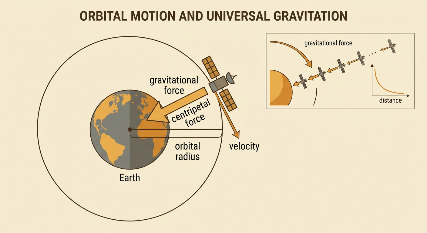
Newton explained Kepler’s patterns using universal gravitation. The gravitational force between masses M and m separated by distance r is F = GMm/r². For a circular orbit, gravity supplies the centripetal force needed to continually turn the satellite’s velocity: GMm/r² = mv²/r. The satellite’s mass cancels, showing that ideal orbital speed at a given radius does not depend on the satellite’s mass. Solving gives v = √(GM/r). Gravity becomes weaker with increasing distance, so more distant circular orbits have lower speeds. For example, the Moon’s average distance from Earth’s center is about 3.84 × 10⁸ meters. Using Earth’s mass in the equation predicts an average orbital speed near 1.02 kilometers per second, close to the observed value. Real orbits can also be affected by other bodies and uneven mass distributions.
Orbital Speed and Period Calculations
For a circular orbit around Earth, speed is v = √(μ/r), where μ = GM = 3.986 × 10¹⁴ cubic meters per second squared and r is measured from Earth’s center. The period is T = 2π√(r³/μ). Consider a satellite 400 kilometers above Earth. Adding Earth’s approximate 6,370-kilometer radius gives r = 6.77 × 10⁶ meters. Substitution gives v ≈ 7.67 kilometers per second and T ≈ 5,550 seconds, or about 92.5 minutes. Function graphs make the relationships visible. The graph of v(r) decreases and gradually flattens as radius increases, while the graph of T(r) rises more steeply as radius increases. These symbolic functions allow scientists to predict an orbit and check whether computational results have reasonable intercepts, domains, and overall trends.

Satellite Orbits and Geospatial Applications
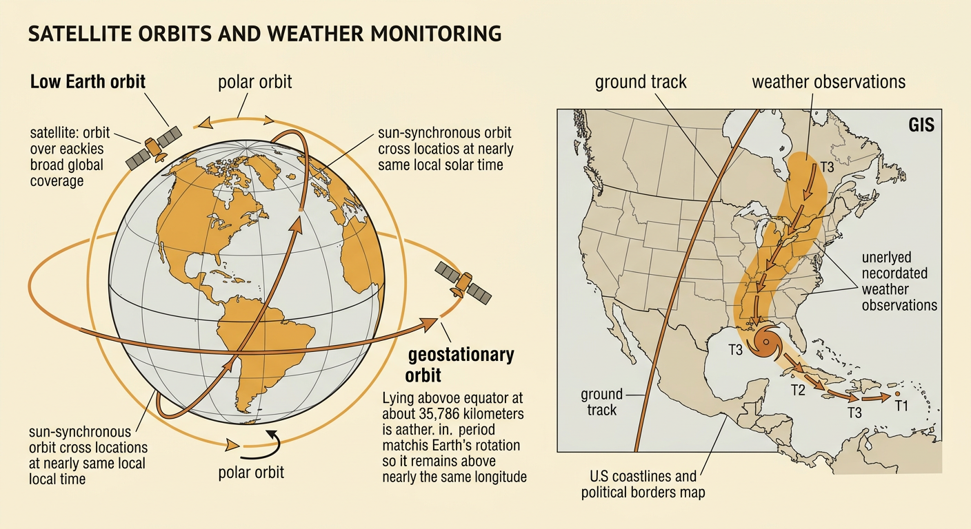
Satellite orbit selection depends on the observation or communication task. Low Earth orbit supports detailed imaging because satellites pass relatively close to Earth. Polar and sun-synchronous orbits allow repeated coverage of much of the planet under similar lighting conditions. Geostationary satellites orbit above the equator at about 35,786 kilometers altitude and match Earth’s rotation, so they remain above nearly the same longitude. For example, GOES weather satellites repeatedly observe the same large region, helping meteorologists track hurricanes and cloud movement. Geographic information systems combine satellite images with coordinates, map layers, and time data. Analysts can compare vegetation, sea ice, urban growth, wildfire smoke, or storm paths across locations and dates. Ground tracks displayed on digital maps also reveal where and when a satellite can collect data or communicate with a ground station.