Testing Statistical Significance with Randomization
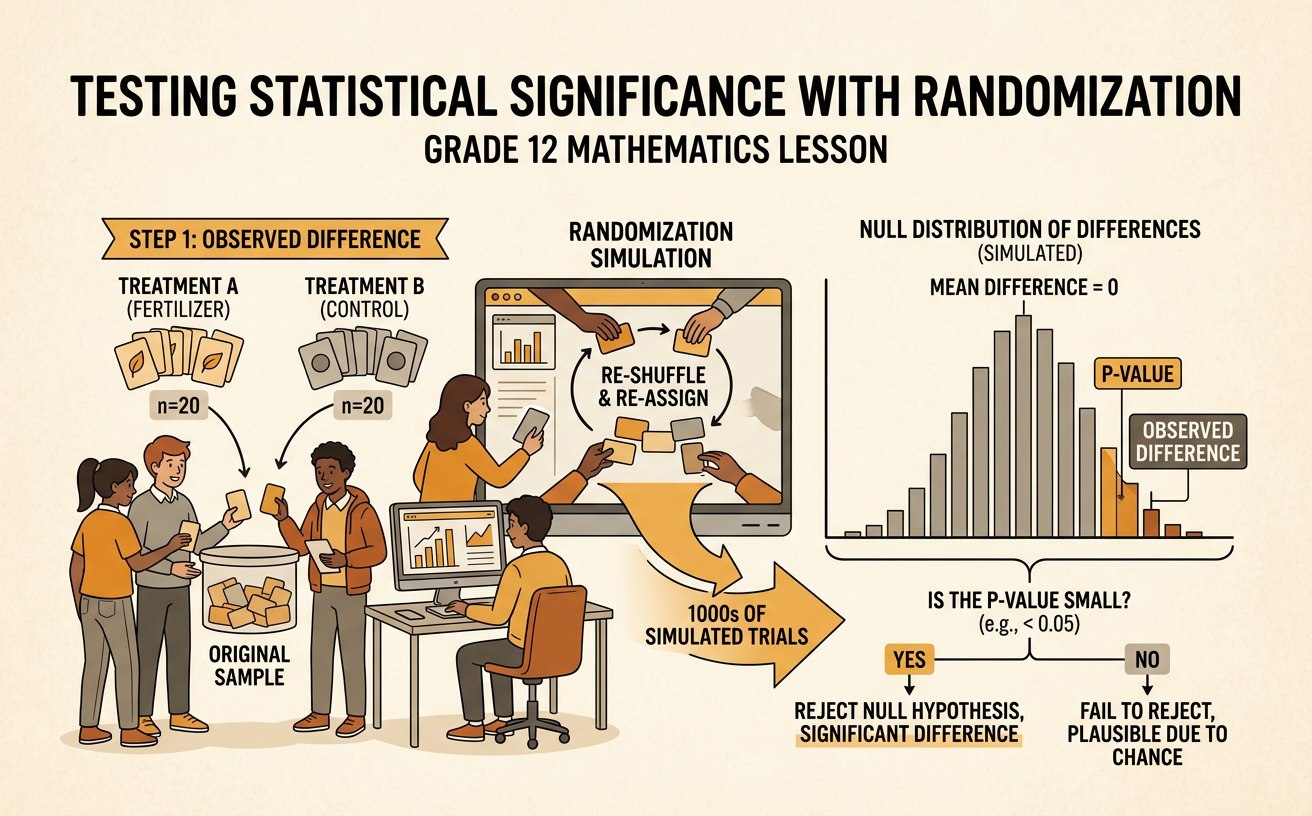
Students use randomization simulations to determine whether an observed difference between two treatment groups is statistically significant or plausibly due to chance.
Illustrations are auto-generated and may be placeholders. They can be refreshed to match the narration.
Formulate the Null Hypothesis
Begin by stating what would be true if the treatment had no effect. Suppose researchers randomly assign 40 similar plants to two fertilizers, with 20 plants receiving Fertilizer A and 20 receiving Fertilizer B. The null hypothesis states that the two fertilizers produce the same mean plant growth in the population. Any difference between the sample means would therefore result from the chance involved in assigning plants to groups. In symbols, the null hypothesis is H₀: μA − μB = 0. A suitable alternative hypothesis is HA: μA − μB ≠ 0, meaning the fertilizers have different effects on mean growth. The hypotheses concern population parameters, not just the observed sample means. A randomization test begins by assuming the null hypothesis is true and examining what differences chance alone could produce.

Identify the Observed Difference
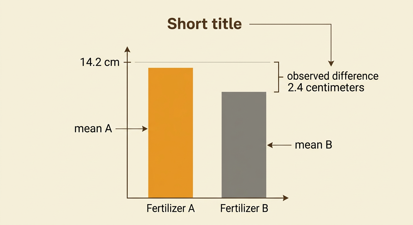
Next, calculate a statistic that compares the treatment groups. After four weeks, suppose the 20 plants given Fertilizer A grew an average of 14.2 centimeters, while the 20 plants given Fertilizer B grew an average of 11.8 centimeters. Define the difference as mean growth for A minus mean growth for B. The observed difference is 14.2 − 11.8 = 2.4 centimeters. Its positive sign indicates that the A group had greater average growth. The order of subtraction must remain consistent throughout the randomization test. The statistic describes the samples, but it does not by itself show that Fertilizer A caused more growth. Researchers must determine whether a difference of 2.4 centimeters would be unusual if the null hypothesis of no treatment effect were true.
Build a Randomization Distribution
To model chance variation under the null hypothesis, keep all 40 recorded growth values but temporarily ignore their original fertilizer labels. Randomly shuffle the labels and assign 20 values to A and 20 to B, preserving the original group sizes. Calculate the shuffled difference, mean A minus mean B, and record it. Repeat this process many times, such as 1,000 random shuffles. Because the null hypothesis treats the fertilizers as equally effective, the labels are interchangeable, and the simulated differences should cluster around zero. Some shuffles will produce positive differences and others negative differences. A histogram of all simulated differences forms the randomization distribution. This distribution shows the differences that random assignment could plausibly create when there is no genuine fertilizer effect. The original observed difference is not included as evidence repeatedly; it is compared with this simulated reference distribution.

Estimate the P-Value
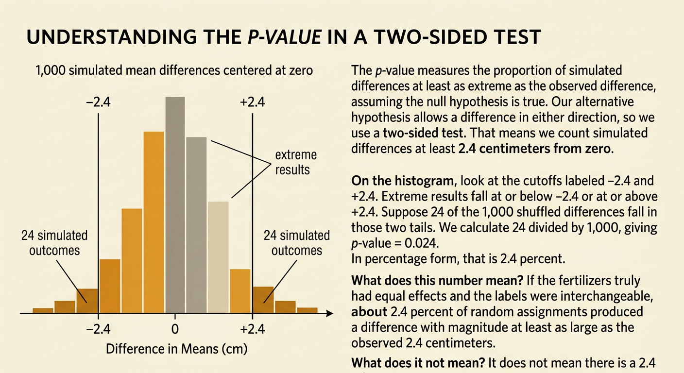
The p-value is the proportion of simulated differences at least as extreme as the observed difference, assuming the null hypothesis is true. Because the alternative hypothesis says the fertilizers differ in either direction, use a two-sided test. Count simulated differences that are at least 2.4 centimeters from zero: differences greater than or equal to 2.4 or less than or equal to −2.4. Suppose 24 of the 1,000 shuffled differences meet this condition. The estimated p-value is 24 ÷ 1,000 = 0.024. This means that about 2.4% of the random assignments produced a difference with magnitude at least as large as 2.4 centimeters when treatment labels were interchangeable. The p-value is not the probability that the null hypothesis is true. It measures how unusual the observed result is under the null model.
Draw a Context-Based Conclusion
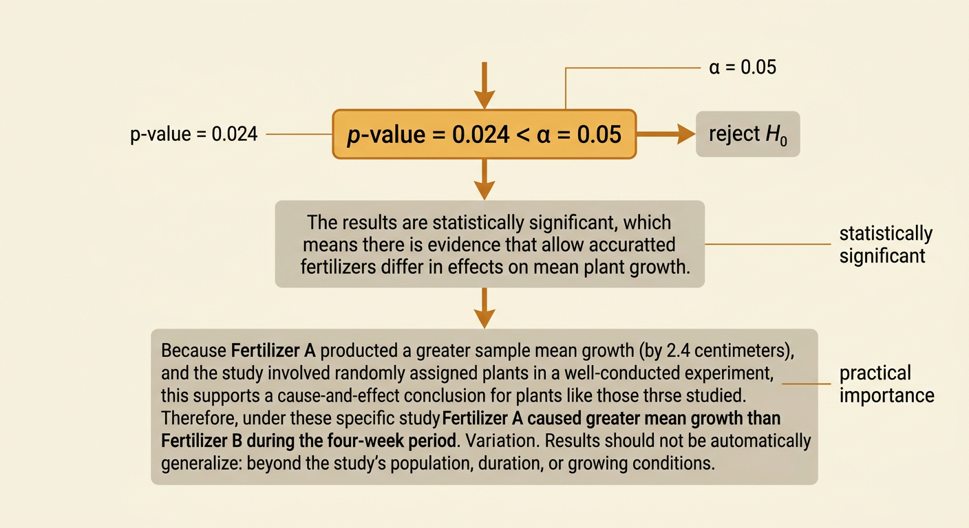
Compare the p-value with a chosen significance level, commonly α = 0.05. Here, 0.024 is less than 0.05, so reject the null hypothesis. The observed 2.4-centimeter difference would be relatively unusual if the fertilizers truly had equal effects. Therefore, the experiment provides statistically significant evidence that the two fertilizers differ in their effects on mean plant growth. Because plants were randomly assigned to treatments, a well-conducted experiment supports a cause-and-effect conclusion for plants like those studied: Fertilizer A caused greater mean growth than Fertilizer B during the four-week period. The conclusion should remain tied to the study’s conditions and population. Statistical significance also does not automatically establish practical importance; researchers should consider whether an average increase of 2.4 centimeters is useful enough to matter in the intended agricultural setting.