The Great Smog of London: Industrial Pollution and Public Policy
Students examine historical accounts and pollution data to explain how industrialization, weather conditions, and public pressure led to Britain’s Clean Air Act of 1956.

Illustrations are auto-generated and may be placeholders. They can be refreshed to match the narration.
Industrial London and Coal Dependence
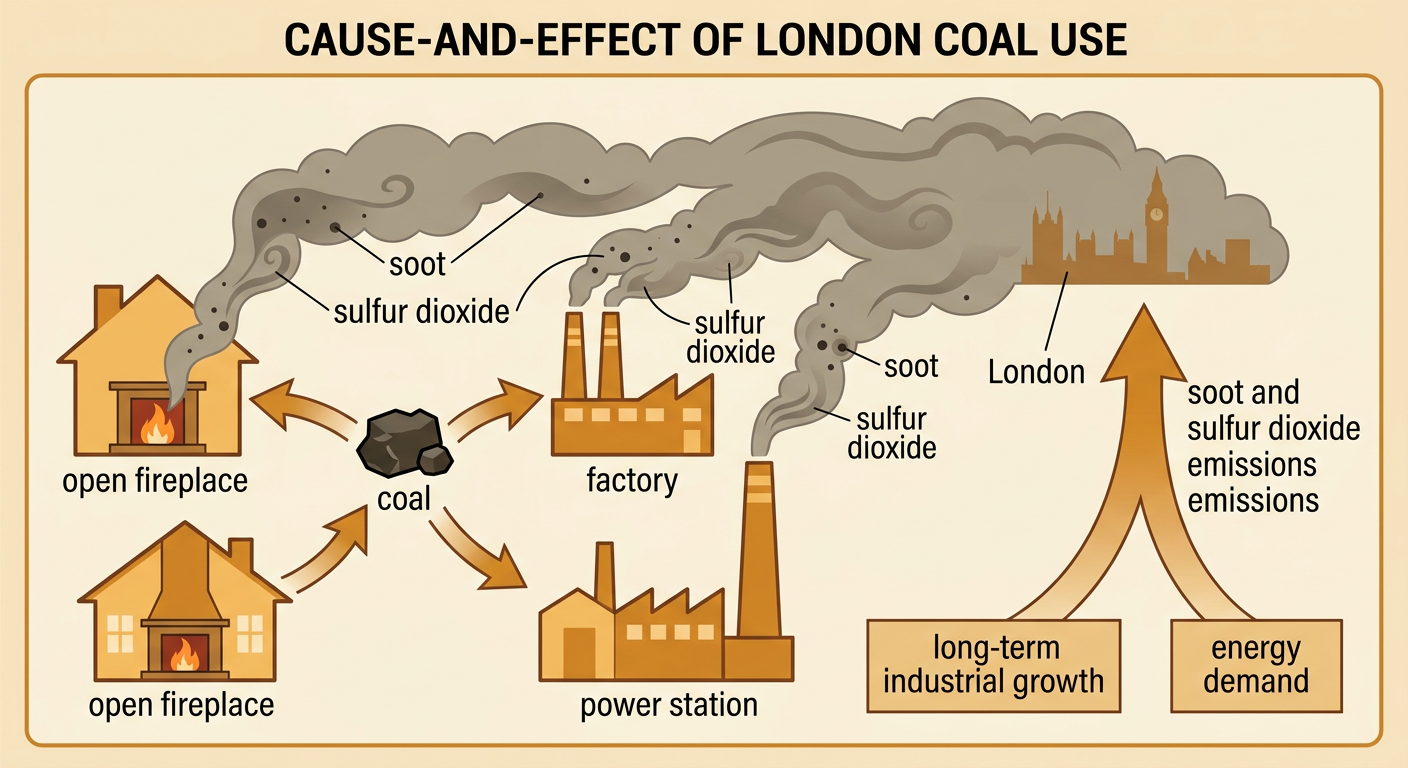
By the early 1950s, London depended heavily on coal for heating homes, generating electricity, powering industry, and supporting transportation. Cheap, low-grade coal often contained sulfur and produced thick smoke when burned. Many households used open fireplaces, so thousands of chimneys released soot and sulfur dioxide close to street level. Factories and coal-fired power stations added more pollution. This dependence was an underlying cause of the Great Smog because it developed over decades of industrialization and urban growth. For example, during cold weather, Londoners burned extra coal to heat poorly insulated homes, sharply increasing emissions. Coal supplied affordable energy and jobs, but its widespread use created serious health and environmental costs that were not fully controlled by existing laws.
Weather Conditions and the 1952 Smog
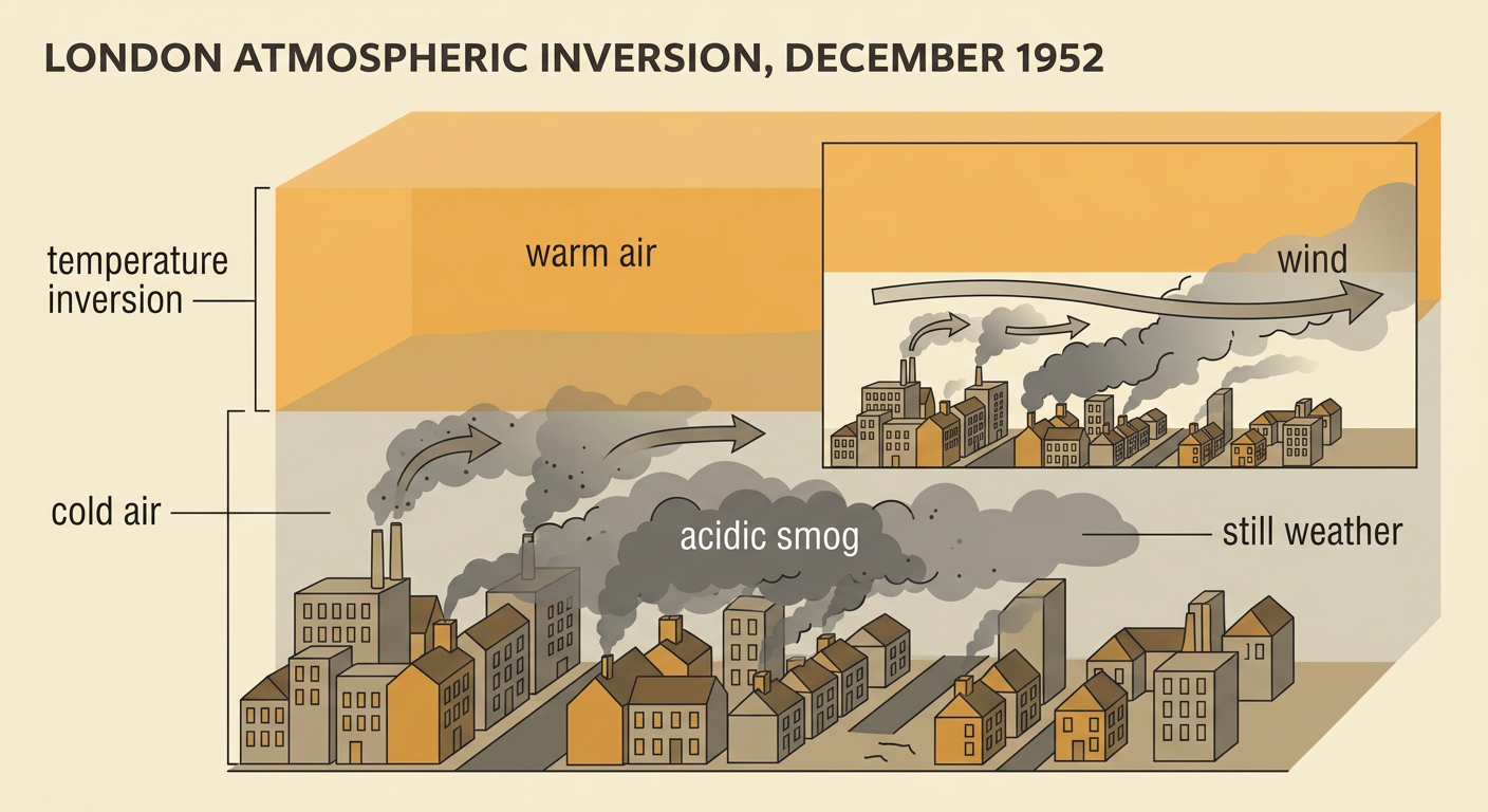
The immediate trigger of the Great Smog was an unusual period of cold, still weather beginning on December 5, 1952. A high-pressure system produced a temperature inversion: cold air remained near the ground while warmer air above acted like a lid. With very little wind, smoke from chimneys could not rise and disperse. Natural fog droplets mixed with soot, sulfur dioxide, and other pollutants, forming a dense, acidic smog. Residents burned more coal because temperatures were low, adding pollution to the trapped air. The smog lasted about five days, until changing weather brought wind that cleared it. The inversion did not create the emissions, but it concentrated existing pollution. Thus, coal dependence was an underlying cause, while the cold and inversion were immediate conditions.
Reading Pollution and Mortality Data
Pollution and mortality records help historians measure the smog’s effects. A time-series graph can place dates on the horizontal axis and show pollution concentration and daily deaths on separate vertical scales. During the smog, measurements of smoke and sulfur dioxide rose sharply, followed by a major increase in deaths. Early government reports identified about 4,000 excess deaths, while later research estimated that the total may have reached roughly 12,000 when deaths in the following months were included. Students can also create a scatterplot with daily pollution levels on one axis and daily deaths on the other. An upward pattern would show a positive association between the variables. However, the graph alone does not prove causation; medical reports, timing, and evidence about respiratory and cardiovascular illness strengthen the explanation.

Experiences of London Residents
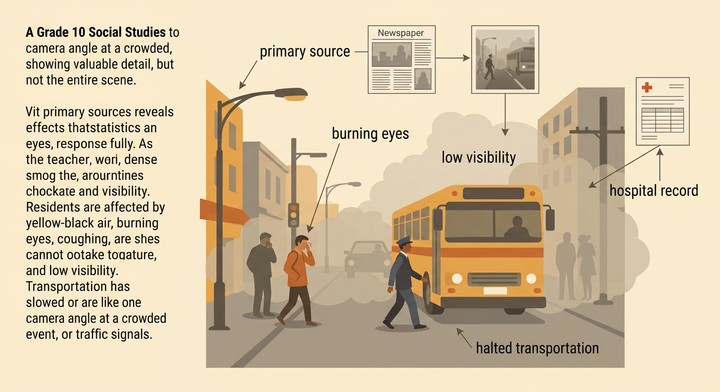
Primary sources reveal how the smog affected daily life in ways that statistics cannot fully capture. Residents described yellow-black air, burning eyes, coughing, and visibility reduced to only a few feet in some places. Transportation slowed or stopped because drivers could not see traffic signals or road edges. Some bus conductors reportedly walked in front of vehicles to guide drivers, while indoor events were disrupted when smog entered buildings. Hospitals treated increasing numbers of people with breathing difficulties, especially older adults and people with existing heart or lung conditions. When using an account, students should identify who created it, when it was created, and what details can be confirmed by other sources. For example, a newspaper report about halted transportation can be compared with transit records and photographs from the same dates.
Government Debate and the Clean Air Act
The disaster increased public pressure for national action, but reform was not immediate. Some officials questioned whether pollution alone caused the deaths, while others worried that cleaner fuels and new equipment would be expensive. The government appointed a committee led by Hugh Beaver to investigate air pollution and recommend solutions. Its findings helped build support for the Clean Air Act of 1956. The law restricted emissions of dark smoke, allowed local governments to create smoke control areas, and supported household conversion from coal fires to cleaner heating systems through grants. It also encouraged better control of industrial emissions. For example, in a smoke control area, residents could no longer freely burn smoky coal in ordinary fireplaces. The act represented a policy response shaped by scientific evidence, public pressure, economic debate, and the visible consequences of the 1952 disaster.

Evaluating the Impact of Reform
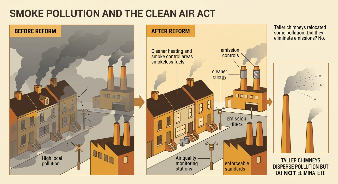
The Clean Air Act of 1956 reduced smoke pollution, but its results should be evaluated over time rather than judged by one event. Smoke control areas and cleaner household fuels reduced the soot released in many urban neighborhoods. Later laws, including the Clean Air Act of 1968, strengthened controls on industrial emissions. London still experienced a serious smog episode in 1962, showing that implementation and technological change took time. A useful evaluation compares pollution measurements, severe-smog days, and respiratory deaths before and after the reforms while also considering changes in fuel use and industry. Some solutions had limitations: taller chimneys reduced local concentrations but could transport pollutants to other places rather than eliminate them. An improved solution would combine cleaner energy, emission filters, building efficiency, monitoring, and enforceable standards so that pollution is prevented instead of merely relocated.