
Understanding Sampling Distributions and Sampling Variability
Students use repeated random samples to examine how sample statistics vary and why larger samples generally produce more consistent estimates of a population parameter.
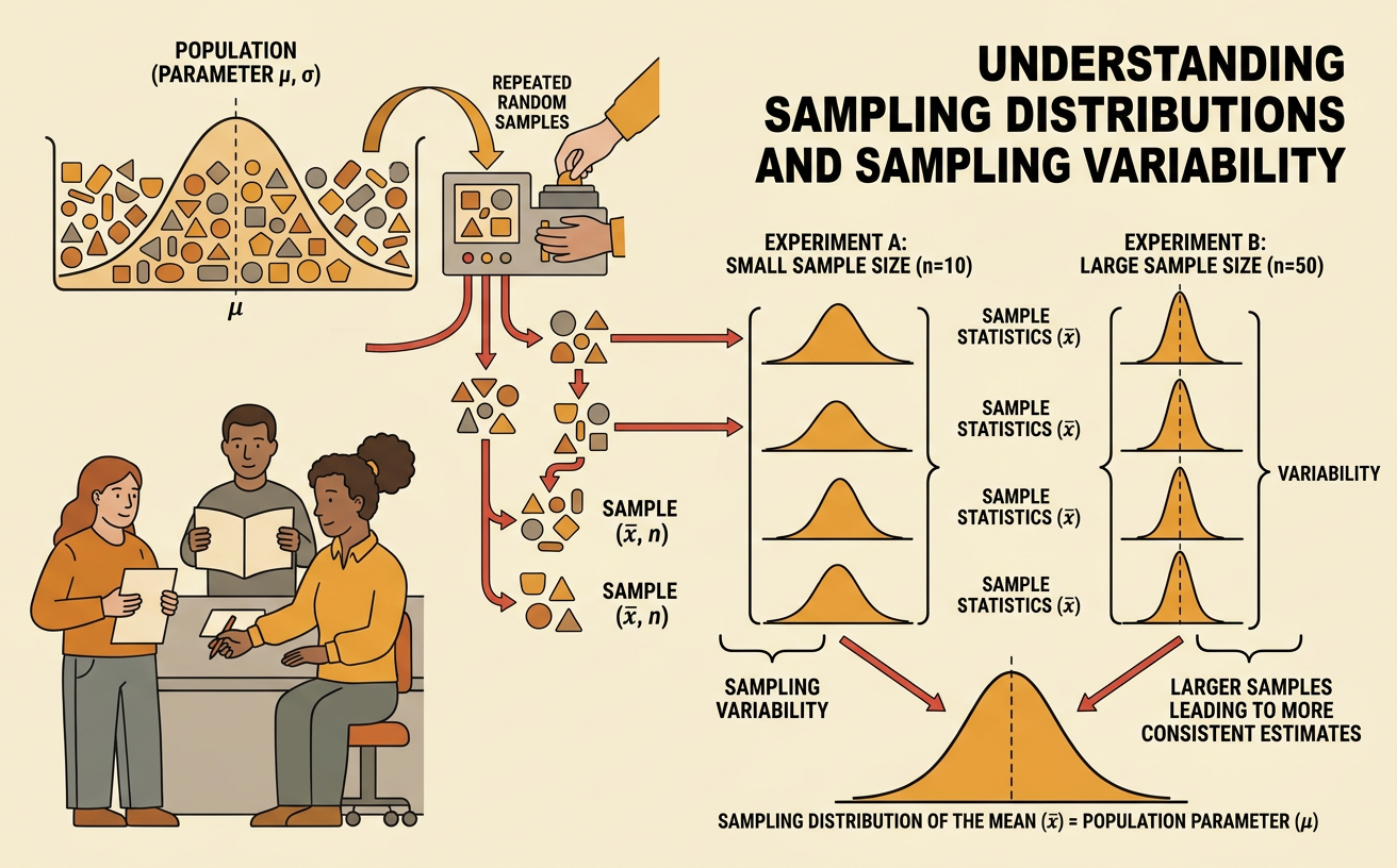
Illustrations are auto-generated and may be placeholders. They can be refreshed to match the narration.
Population Parameters and Sample Statistics
A population is the entire group we want to understand, while a sample is a smaller group selected from that population. A population parameter is a numerical feature of the population, such as its true mean or proportion. A sample statistic is calculated from sample data and is used to estimate the unknown parameter. For example, suppose a school district wants to know the mean number of hours its 12th-grade students sleep each night. The mean for every 12th grader in the district is the population parameter. If researchers randomly select 100 students and find a sample mean of 6.9 hours, then 6.9 is a sample statistic. A different random sample would probably produce a somewhat different mean. Random sampling helps make the sample representative and supports reasonable inferences about the population.

Simulating Repeated Random Samples
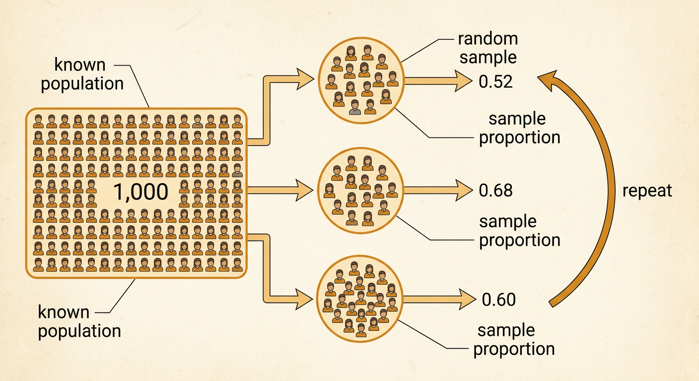
A simulation can model what happens when many random samples are drawn from the same population. Begin with a known population, select a random sample of a fixed size, calculate a statistic, and record it. Then replace the observations and repeat the process many times. Suppose a population contains 1,000 students, and 60 percent prefer a later school start time. A computer can randomly choose 25 students and calculate the sample proportion who prefer a later start. One sample might produce 0.52, another 0.68, and another 0.60. After hundreds of repetitions, the recorded proportions reveal how much the statistic changes from sample to sample. This repeated-sampling process does not mean surveying the same students repeatedly; it represents drawing many possible random samples using the same method and sample size.
Building a Sampling Distribution
A sampling distribution is the distribution of a statistic from all possible random samples of a given size, or from many samples generated by simulation. It is not a distribution of individual data values. To build one, place each calculated statistic on a number line or group the statistics into intervals, then display their frequencies in a dot plot or histogram. For example, researchers might draw 500 random samples of 25 students from a population in which 60 percent prefer a later start time. Each sample contributes one sample proportion to the graph. The resulting sampling distribution may have a mound-like shape, with many proportions near 0.60 and fewer near values such as 0.40 or 0.80. This graph summarizes the possible values of the statistic and how frequently each value occurs.

Interpreting Center and Variability
The center of a sampling distribution shows the typical value of the sample statistic. With a sound random-sampling method, the distribution of sample proportions is generally centered at the population proportion, and the distribution of sample means is generally centered at the population mean. This makes these statistics useful estimators. Variability describes how far sample statistics typically fall from that center. In the school start-time example, a sampling distribution centered near 0.60 indicates that the sample proportion does not systematically overestimate or underestimate the population proportion. However, individual samples might produce 0.52 or 0.68 because of sampling variability. Sampling variability is the natural variation caused by selecting different random samples. It is not necessarily a mistake. Statistics close to the center are more common, while statistics far from the center are usually less common.

Examining the Effect of Sample Size
Larger random samples generally produce statistics with less sampling variability because they include more information from the population. Consider estimating the proportion of students who prefer a later school start. If repeated samples contain only 25 students, the sample proportions may range widely, perhaps from 0.36 to 0.84. If repeated samples contain 200 students, most proportions will be much closer to the true value of 0.60. The centers of both sampling distributions should remain near 0.60, but the distribution for samples of 200 will be narrower. Increasing sample size does not guarantee that one particular sample will be accurate, and it does not correct a biased sampling method. However, when samples are selected randomly, a larger sample size usually gives a more precise estimate of the population parameter and reduces the effect of chance differences among samples.
