
Using Normal Distributions to Estimate Population Percentages
Students use the mean, standard deviation, and properties of the normal distribution to estimate population percentages and interpret results in context.

Illustrations are auto-generated and may be placeholders. They can be refreshed to match the narration.
Recognizing a Normal Distribution
A normal distribution is a continuous, bell-shaped distribution that is symmetric about its mean. Most values cluster near the center, and fewer values appear as distance from the mean increases. In a perfectly normal distribution, the mean, median, and mode are equal. To decide whether a data set is reasonably modeled by a normal distribution, examine a histogram or dot plot for one central peak, approximate symmetry, and no extreme gaps or outliers. For example, the heights of 1,000 adult women might form an approximately normal distribution centered near 64 inches. However, household incomes are often skewed right because a small number of incomes are extremely high. Such income data should not be modeled as normal without careful justification.

Mean and Standard Deviation Review
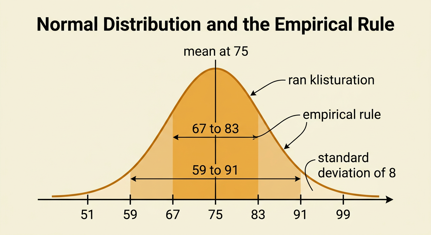
The mean describes the center of a data set, while the standard deviation describes how far values typically spread from the mean. A small standard deviation produces a narrow normal curve; a large standard deviation produces a wider curve. For a normal distribution, about 68% of values lie within one standard deviation of the mean, about 95% lie within two, and about 99.7% lie within three. Suppose exam scores have a mean of 75 points and a standard deviation of 8 points. About 68% of scores are expected between 67 and 83 because 75 minus 8 is 67 and 75 plus 8 is 83. About 95% are expected between 59 and 91, assuming the normal model is appropriate.
Standardizing Values with z-Scores
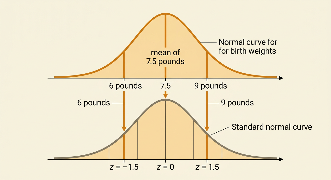
A z-score states how many standard deviations a value is above or below the mean. Calculate it using z = (x − mean) ÷ standard deviation. Positive z-scores represent values above the mean, negative z-scores represent values below the mean, and a z-score of zero represents the mean. Suppose birth weights are approximately normal with a mean of 7.5 pounds and a standard deviation of 1.0 pound. A weight of 9 pounds has z = (9 − 7.5) ÷ 1.0 = 1.5, so it is 1.5 standard deviations above the mean. A weight of 6 pounds has z = (6 − 7.5) ÷ 1.0 = −1.5. Converting values to z-scores allows different normal distributions to be analyzed using the same standard normal curve.
Estimating Percentages Under the Curve
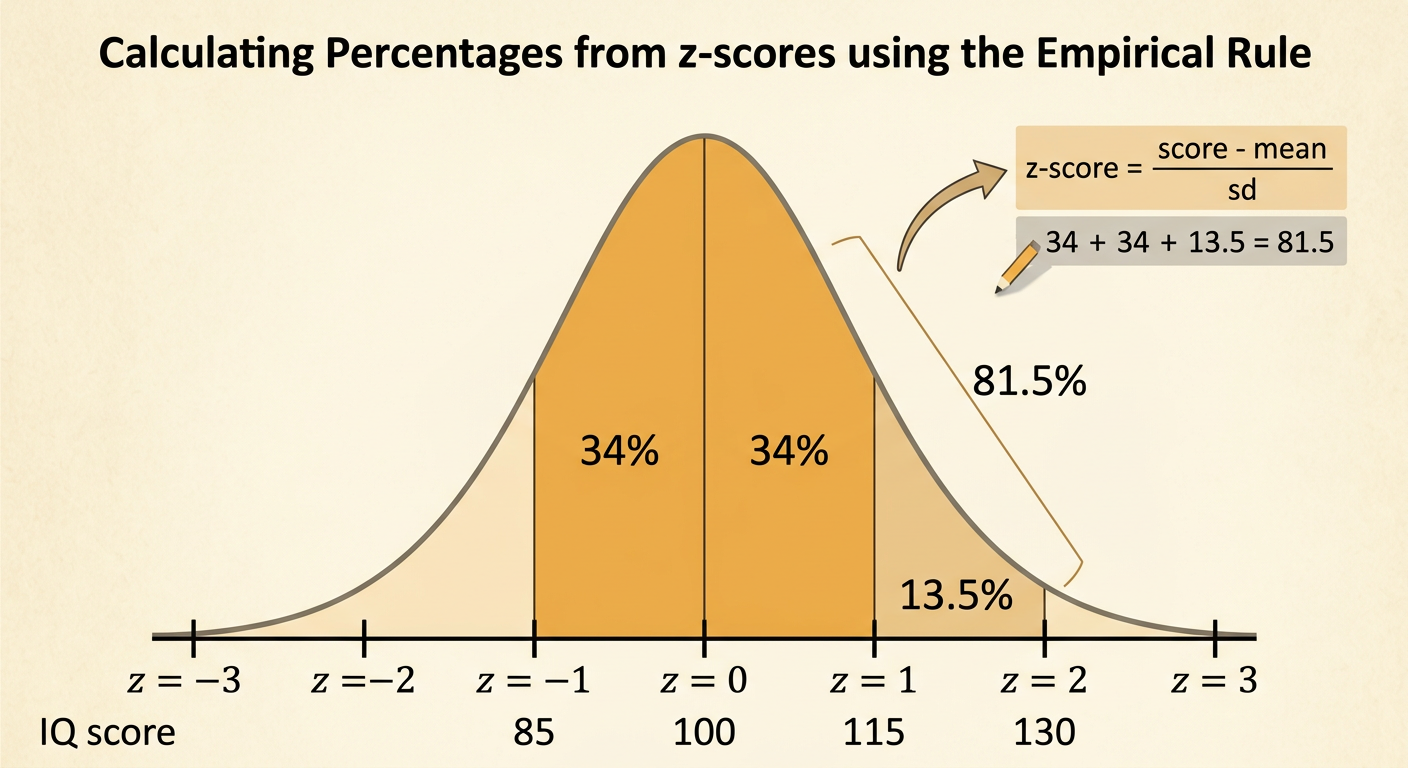
Percentages in a normal distribution correspond to areas under the normal curve. After converting boundary values to z-scores, use the empirical rule, a standard normal table, or technology to find the area in the desired region. Suppose IQ scores are approximately normal with a mean of 100 and a standard deviation of 15. For scores from 85 to 130, the z-scores are −1 and 2. The empirical rule divides the curve into useful sections: about 34% lies from z = −1 to 0, 34% from 0 to 1, and 13.5% from 1 to 2. Adding these areas gives about 81.5%. Therefore, approximately 81.5% of the population is expected to have IQ scores between 85 and 130.
Interpreting Estimates in Context
A normal-model percentage should be stated in terms of the population and the variable being measured. It can also be used to estimate a count by multiplying the percentage by the population size. Suppose the lifetimes of a certain light bulb model are approximately normal with a mean of 1,200 hours and a standard deviation of 100 hours. About 2.5% of lifetimes should exceed 1,400 hours because 1,400 is two standard deviations above the mean and about 2.5% lies above that point. Among 8,000 bulbs, the estimated count is 0.025 × 8,000 = 200 bulbs. This is an estimate, not a guarantee. If the lifetime data are skewed, contain outliers, or come from a nonrepresentative sample, the normal-model estimate may be unreliable.
