
Variation and Word Problems
Students model direct, inverse, joint, and partial variation and use resulting equations to solve practical problems.
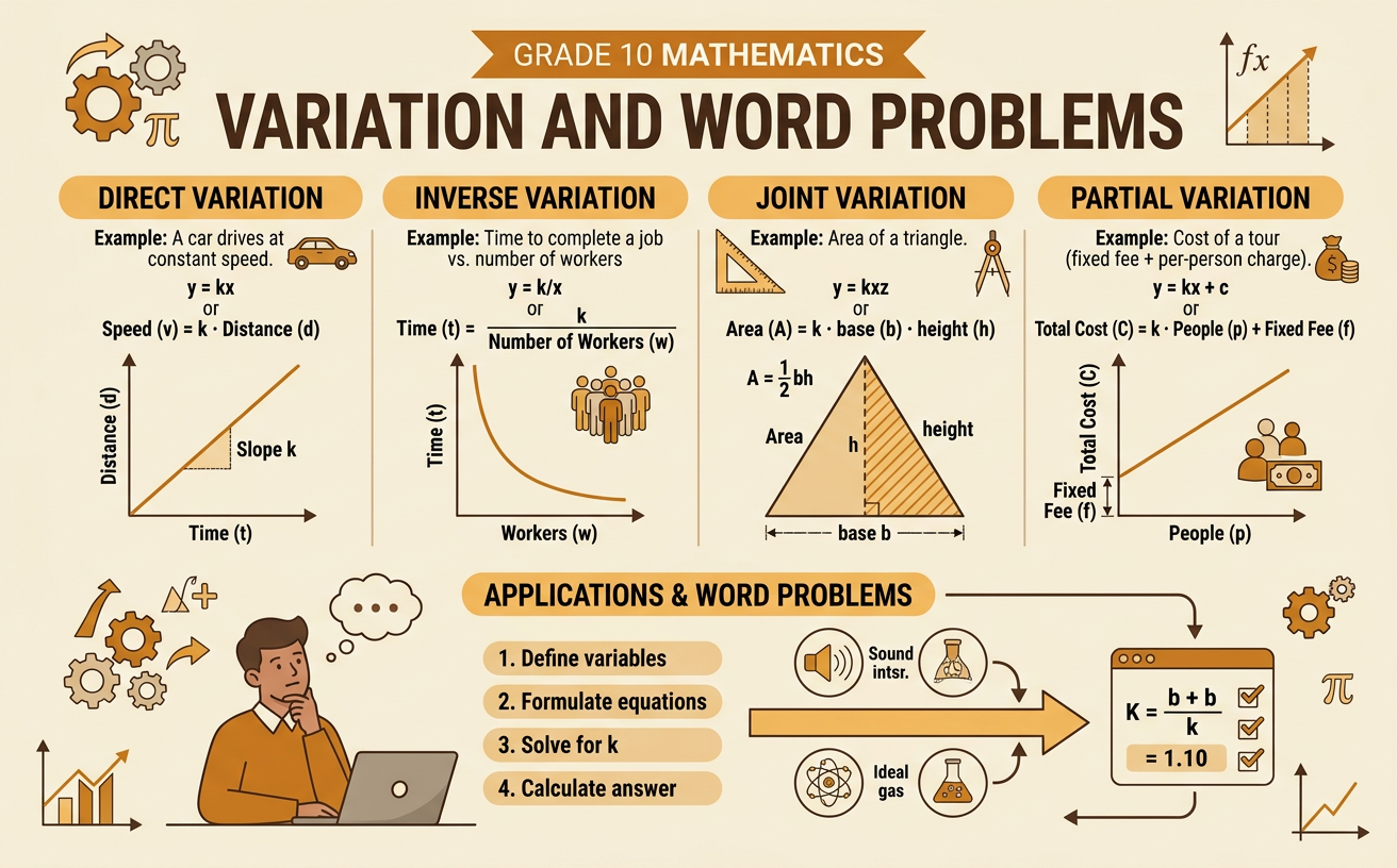
Illustrations are auto-generated and may be placeholders. They can be refreshed to match the narration.
Direct Variation
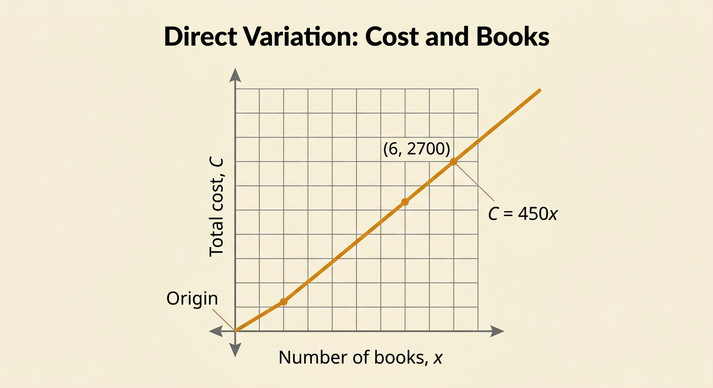
Direct variation occurs when one quantity changes in a constant ratio to another. It is modeled by y = kx, where k is the constant of variation. The graph is a straight line through the origin because y = 0 when x = 0. For example, suppose exercise books cost ₦450 each. If x is the number of books and C is the total cost, then C = 450x. Here, 450 is the constant of variation. For 6 books, C = 450 × 6 = ₦2,700. Also, C/x = 450 for every nonzero value of x. Doubling the number of books doubles the cost, while tripling the number triples the cost.
Inverse Variation
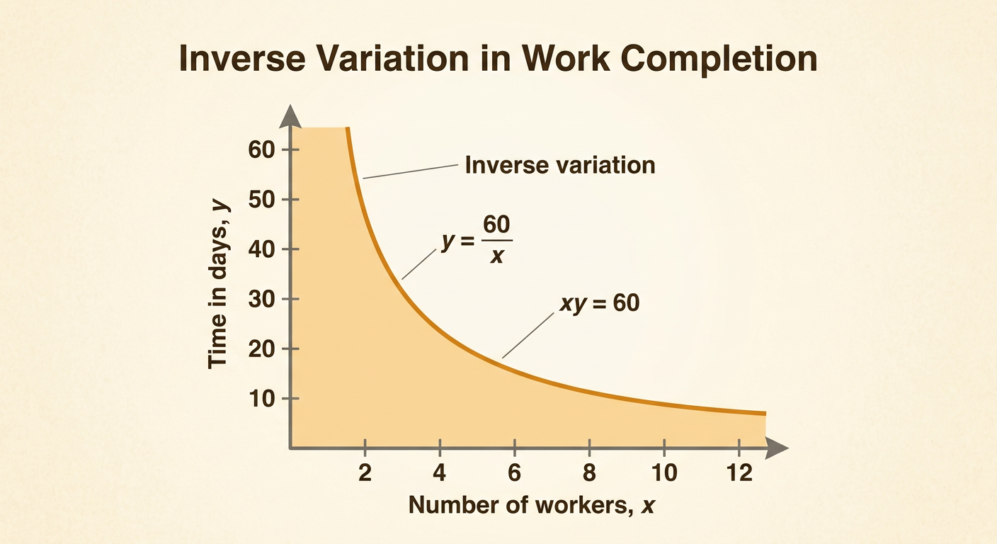
Inverse variation occurs when one quantity increases as another decreases so that their product remains constant. It is modeled by y = k/x, or xy = k, where x is not zero. For example, the time needed to complete a job may vary inversely with the number of workers, provided all workers work at the same rate. If 6 workers complete a task in 10 days, then k = 6 × 10 = 60 worker-days. With 12 workers, the time is y = 60/12 = 5 days. Thus, doubling the number of workers halves the time. The graph of a positive inverse variation is a curved hyperbola that approaches, but does not touch, either axis.
Joint Variation
Joint variation occurs when one quantity varies directly with the product of two or more other quantities. If y varies jointly with x and z, the equation is y = kxz. A rectangular box provides a familiar example: its volume V varies jointly with its length l, width w, and height h. Therefore, V = klwh. For ordinary volume measurement, k = 1, so V = lwh. A box with length 8 cm, width 5 cm, and height 3 cm has volume V = 1 × 8 × 5 × 3 = 120 cm3. If only the height doubles while the other dimensions stay fixed, the volume also doubles. Joint variation requires every listed varying factor to appear as a product.
Partial Variation
Partial variation combines a fixed amount with an amount that varies directly. Its usual form is y = a + bx, where a is the fixed value and b is the rate of change. Unlike a direct variation graph, its graph does not usually pass through the origin. For example, a delivery service may charge a fixed booking fee of ₦500 plus ₦150 for each kilometer traveled. If d is the distance and C is the total charge, then C = 500 + 150d. For a journey of 8 kilometers, C = 500 + 150(8) = 500 + 1,200 = ₦1,700. The value 500 is the vertical intercept, while 150 is the cost added per kilometer.
Finding the Constant
To find a constant of variation, first write the correct variation equation, substitute the known values, and solve for k. For direct variation, y = kx, so k = y/x. For inverse variation, y = k/x, so k = xy. For joint variation, y = kxz, so k = y/(xz). Suppose P varies jointly with m and n, and P = 72 when m = 4 and n = 3. Substitute to obtain 72 = k(4)(3). Therefore, 72 = 12k and k = 6. The complete model is P = 6mn. If m = 5 and n = 2, then P = 6(5)(2) = 60. Always include the constant before using the equation to predict another value.
Practical Applications
Variation models help describe costs, travel, work, production, and measurements. Begin by identifying how the quantities are related. The phrase “at a constant rate” often suggests direct variation, “fixed fee plus” suggests partial variation, and “more workers require less time” suggests inverse variation. Consider a motorcycle delivery with a fixed charge of ₦700 and a distance charge of ₦180 per kilometer. The cost C for d kilometers is C = 700 + 180d. For 15 kilometers, C = 700 + 180(15) = ₦3,400. If a customer can spend ₦4,600, solve 4,600 = 700 + 180d. Then 3,900 = 180d, so d = 21.67 kilometers, approximately. The model allows both prediction and decision-making.